by Andy Meyer

Introduction

This article describes a project that used the statistical programming language R to generate reports about electronic usage and spending. This project had three main goals. First, to automate and systematize the process of gathering, compiling, and communicating data about electronic resource usage. Second, to increase library staff capacity for data science. Third, to provide a shareable framework and model for other libraries to use when dealing with data intensive projects. This project focused on electronic resource usage information in the form of Counter Reports but can be extended to manage and communicate data from a variety of other library systems or other data sources.

Background

With library budgets shrinking and the cost of online resources growing, many libraries must critically examine electronic resource usage and related costs to make responsible collection development decisions. Yet gathering this information, transforming the raw data into something usable, and communicating relevant information is a difficult and labor intensive process. The goal for this particular project is to provide electronic resource usage information to other library staff to aid collection development decisions. However, this approach could be extended to deal with other data and communicate those results to a wide variety of stakeholders.

R and the Tidyverse

R is an open source programming language freely available under the GNU General Public License. R excels in statistical computing and is growing in popularity across many disciplines. R enjoys a large and active user community as well as a number of packages that extend the basic functions of R. The growing popularity of R, the strong and active user community, the ability to do reproducible and rigorous data analysis, and the open nature of R make this an excellent option for many library applications. Furthermore, developing staff expertise in R may position the library to take on additional roles in data management and create new connections on campus.

The Tidyverse is a set of R packages that “share a common philosophy of data and R programming and are designed to work together naturally.”[1] The Tidyverse is a great place to begin learning R because these packages are widely adopted and relatively intuitive. There is also an abundance of high quality documentation that is freely available online.

Counter Reports

COUNTER is a non-profit organization that provides libraries, publishers, and vendors a Code of Practice and set of definitions that facilitates the standard and consistent way to look at electronic resource usage.[2] The project described in this paper uses the Database 1 report. These reports include the number of regular searches, result clicks, record views, federated/automated searches by Month and by Database. This is a standard report that most electronic resource vendors provide; details and definitions are available on the counter website.[3] This project uses revision 4 reports but the general approach outlined here could easily be extended to include other revisions and/or other counter-complaint reports.

Code Structure and Style

This project approaches data science following the model proposed by Garrett Grolemund and Hadley Wickham in “R for Data Science”. The code is divided and structured into three discrete stages:

1. Import and Tidy
2. Transform, Visualize, and Model
3. Communicate

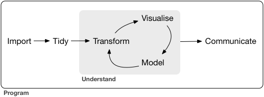
Figure 1. Model of the tidyverse approach to data science from from Grolemund, Garrett, and Hadley Wickham. “R for Data Science” http://r4ds.had.co.nz/introduction.html.[4]

Following another tenet of the Tidyverse, this project has adopted a functional approach to R. This approach limits redundant code and makes the meaning of the code more transparent. In terms of style, the code is written for clarity and simplicity; it is not written to optimize performance. The hope is that the variable and function names as well as the comments allow others to easily use and adapt this code to their local institutional needs. Lastly, this project makes extensive use of the pipe function in R. As a core member of the Tidyverse, this function makes R code more readable and beautiful by combining complex operations without requiring nested functions. The book “R for Data Science” offers a very clear explanation of the pipe function.[5]

Tidy Data

Before moving on, a note about terminology. In the context of the Tidyverse and throughout this paper, the word “tidy” carries a specific and technical definition. The goal of tidy data is to create an underlying structure that makes various types of transformation easier. Hadley Wickham offers this definition of tidy data:

“Tidy data is a standard way of mapping the meaning of a dataset to its structure. A dataset is messy or tidy depending on how rows, columns and tables are matched up with observations, variables and types. In tidy data:

1. Each variable forms a column.
2. Each observation forms a row.
3. Each type of observational unit forms a table.

Messy data is any other arrangement of the data.”[6]

According to this definition, COUNTER-compliant reports, although standardized, are messy because the structure of the data – the column and row arrangement – does not correspond with the observations and variables. The process of tidying data begins by identifying the variables. For COUNTER-compliant database report 1, the variables are:

• Database
• Publisher
• Platform
• User Activity
• Date (expressed as Month-Year)
• Usage

Looking at data from a sample report, we can see that while the report is standardized the data is messy because each row contains many observations.

database Report 1 (r4)	Total Searches, Result Clicks and Record Views by Month and Database
Period covered by Report:
2015-01-01 to 2015-12-31
date run:
database	publisher	platform	user Activity	reporting Period total	jan- 2015	feb- 2015	mar-2015	apr-2015	may- 2015	jun- 2015
database A	publisher X	platform Z	regular Searches	13811	758	1884	1686	1951	601	186
database A	publisher X	platform Z	searches – federated and automated	988	49	163	108	145	60	16
database A	publisher X	platform Z	result clicks	10719	611	1562	1277	1609	531	181
database A	publisher X	platform Z	record views	1032	80	223	173	177	50	31

Conveying this data in a tidy dataframe would keep the Database, Publisher, Platform, and User Activity columns and add columns for Date and Usage.

database	publisher	platform	user_Activity	date	usage
database A	publisher X	platform Z	regular Searches	jan-15	758
database A	publisher X	platform Z	searches – federated and automated	jan-15	49
database A	publisher X	platform Z	result clicks	jan-15	611
database A	publisher X	platform Z	record views	jan-15	80
database A	publisher X	platform Z	regular Searches	feb-15	1884
database A	publisher X	platform Z	searches – federated and automated	feb-15	163
database A	publisher X	platform Z	result clicks	feb-15	1562
database A	publisher X	platform Z	record views	feb-15	223
database A	publisher X	platform Z	regular Searches	mar-15	1686
database A	publisher X	platform Z	searches – federated and automated	mar-15	108
database A	publisher X	platform Z	result clicks	mar-15	1277
database A	publisher X	platform Z	record views	mar-15	173
database A	publisher X	platform Z	regular Searches	apr-15	1951
database A	publisher X	platform Z	searches – federated and automated	apr-15	145
database A	publisher X	platform Z	result clicks	apr-15	1609
database A	publisher X	platform Z	record views	apr-15	177
database A	publisher X	platform Z	regular Searches	may-15	601
database A	publisher X	platform Z	searches – federated and automated	may-15	60
database A	publisher X	platform Z	result clicks	may-15	531
database A	publisher X	platform Z	record views	may-15	50
database A	publisher X	platform Z	regular Searches	jun-15	186
database A	publisher X	platform Z	searches – federated and automated	jun-15	16
database A	publisher X	platform Z	result clicks	jun-15	181
database A	publisher X	platform Z	record views	jun-15	31

The data in this table is tidy because all of the variables are in columns and each observation is a row.

Code Overview

All of the code for this project lives on Github: https://github.com/ameyer24/LearningR/tree/master/Electronic%20Resources

Setup

As a preliminary step, this project includes a file that sets up the rest of the process by loading the appropriate packages and by setting up the folder structure.

###############################################################################
# Loading Packages ____________________________________________________________
###############################################################################

library(tidyverse)
library(readxl)
library(lubridate)
library(mosaic)
library(zoo)
library(scales)
library(knitr)

###############################################################################
# Setting Up  Working Directory _______________________________________________
###############################################################################

getwd()
DB1_folder <- "./DB1_reports"
output_folder <- "./outputs"

The library commands load the appropriate packages that are required in this project. If the packages are not installed, you will first need to install the packages. The “Setting Up Working Directory” section sets relative file paths to the inputs folder as well as output folder. This definitions could be changed to explicit file paths to meet local needs.

Import and Tidy

The first step of this project is to import the data from all the files from the folder defined above and create a single tidy dataframe in R. This process might be complicated by a variety of file formats and inconsistent data ranges. To address these problems, the functions in this project can handle COUNTER-compliant reports as both CSV and Excel files while providing a generalizable framework for other file types. The functions can also de-duplicate the usage data so that reports spanning overlapping date ranges will not cause problems. An area of improvement would be to improve handling of missing data. These functions are designed to work with Database Report 1 data but could easily be adapted to import and tidy other COUNTER-compliant reports.

Tidy the Data from Counter Reports

# Transforms data from the standard Counter Format to a tidy dataframe.
tidy_reports <- function(df) {
  df %>%
    select(-c(5)) %>%
    gather(Date, Usage, -c(1:4)) %>%
    mutate(Date = as.yearmon(Date, "%b-%Y")) %>%
    mutate(Usage = as.numeric(Usage)) %>%
    rename("User_Activity" = "User Activity")
}

This function transform data from a COUNTER-compliant format to a tidy dataframe. Looking at each line in detail:

1. select(-c(5)) – This line deletes the 5th column. The Reporting Period Total is not useful within the “Tidyverse” and is therefore removed.
2. gather(Date, Usage, -c(1:4)) – The gather function is the primary way of moving data from a “wide” format into a tidy “long” format. This step keeps the data in columns 1-4 by collapsing all the other columns in key-value pairs. This function creates new variables for the key and value; for COUNTER-compliant reports, the key is the “Date” variable and the value is the “Usage” variable.
3. mutate(Date = as.yearmon(Date, "%b-%Y")) The mutate function adds a new variable from existing variables; here we update the “Date” variable by converting that data from a simple character string to the Year-Mon data type.
4. mutate(usage = as.numerIc(usage)) – Similarly, this function converts the Usage data from a character to numeric.
5. rename("User_activity" = "user activity") – Lastly, this function renames the “User Activity” column to avoid the space in the column name; this is probably optional but made life easier while working with the data.

Import the Data from the Files

The function above transforms a dataframe within R; these functions load the data from a specific file and then apply the tidy_reports function defined above.

# This function imports data from CSV files and makes that data tidy.
import_csv <- function(file) {
  file %>%
    read_csv(skip=7, col_names = TRUE) %>%
    tidy_reports()
}
# This function imports data from Excel files and makes that data tidy.
import_excel <- function(file) {
  file %>%
    read_excel(skip=7, col_names = TRUE) %>%
    tidy_reports()
}

These functions accept a single file as a parameter and import that data by calling the appropriate reading function. Both processes skip the first 7 lines because those lines do not contain relevant information for this analysis and then tidy the data using the function defined above. It is somewhat inelegant to have two functions that do essentially the same thing but keeping the two function separate improves the readability of the code and is effective, conceptually simple, and easily extendable. A generalized import function would also be an improvement.

Loading and Tidying

This phase of the project now has functions that can load a file and tidy the data; we now need a function that can apply these functions to all the files in a given folder.

# These functions load DB1 reports from a given folder.
load_csv <- function(path) { 
  csv_files <- dir(path, pattern = "*.(CSV|csv)", full.names = TRUE)
  tables <- lapply(csv_files, import_csv)
  do.call(rbind, tables)
}

load_excel <- function(path) { 
  excel_files <- dir(path, pattern = "*.(XL*|xl*)", full.names = TRUE)
  tables <- lapply(excel_files, import_excel)
  do.call(rbind, tables)
}

These functions accept a path to a folder as a parameter and then create a list of file names for files that match a particular pattern. The second line applies the appropriate import function to the list of files. Lastly, the do.call(rbind, tables) line binds together these tables by row.

The Tidy Dataframe

At last, we have the functions needed to import data from every CSV and Excel file in a specified folder and create a single tidy dataframe in R.

DB1_data_csv   <- load_csv(DB1_folder)
DB1_data_excel <- load_excel(DB1_folder)

DB1 <- unique(rbind(DB1_data_csv,DB1_data_excel))

The first two steps create two separate dataframes call DB1_data_csv and DB1_data_excel that contain the data from the respective file formats. The final line combines the data into in a single dataframe called DB1. The unique operation deletes any duplicate observations that may be present in the original usage reports.

Transform and Visualize

After importing and tidying the usage data, the next step in Wickham’s model is to transform, visualize, and model this data. Right now, this project performs basic transformations such as filtering, summarizing, and graphing the data. However, given the tidy structure of the data and the powerful tools that R provides for data transformation, there is an opportunity to build functions that radically transform the data and that allow for new insights. Additionally, given the shared data structures and tools, there are opportunities to share these transformation and visualizations freely and create new sets of best practices.

Like the import and tidy process, this project uses a functional approach to handle transformations and visualizations. The majority of these functions perform transformations on the tidy dataframe created earlier without changing or updating that original dataframe. Rather than exhaustively surveying all possible transformations, this paper will highlight two functions. The first function transformation summarizes the data based on academic terms; the second function uses that summarized data to create a simple barplot.

Transform

summarize_usage_academic_term <- function(DatabaseName,
                                         StartYear,
                                         EndYear,
                                         Action = all_actions){
  DB1 %>%
    filter(Database %in% DatabaseName) %>%
    filter(Date >= StartYear, Date <= EndYear) %>%
    filter(User_Activity %in% Action) %>%
    mutate(Year = year(Date), Month=month(Date)) %>%
    mutate(Academic_Term = derivedFactor(
      "Spring" = (Month==1 | Month==2  | Month==3  | Month==4),
      "Summer" = (Month==5 | Month==6  | Month==7  | Month==8),
      "Fall"   = (Month==9 | Month==10 | Month==11 | Month==12)
    )) %>%
    group_by(Database,User_Activity,Academic_Term,Year) %>%
    summarize(Usage=sum(Usage)) %>%
    rename("User Activity" = "User_Activity")
}

This function accepts four parameters: database name, start year, end year, and action. It uses these parameters as filters to the tidy dataframe by returning only observations that match the parameters. The action parameter is optional and defaults to all actions through a variable defined earlier.

As noted earlier, the mutate function creates new variables from existing variables. In this case, the mutate function creates three new variables from the existing date information: Year, Month, and Academic Term. Strictly speaking it was not necessary to create a new variable for month – the Academic Term could be derived directly from the date – but it has been included in the hopes that it makes the code more accessible. The mutate function that creates the Academic Term variable uses the derivedfactor function from the Mosaic package. The last transformation of the data was to group the data and then summarize the usage data based on academic term.

When this function is applied to our sample data, we get this:

database	user Activity	academic_Term	year	usage
database A	record views	spring	2015	653
database A	record views	spring	2016	147
database A	record views	summer	2015	103
database A	record views	summer	2016	53
database A	record views	fall	2015	276
database A	record views	fall	2016	174
database A	regular Searches	spring	2015	6279
database A	regular Searches	spring	2016	4896
database A	regular Searches	summer	2015	1125
database A	regular Searches	summer	2016	1802
database A	regular Searches	fall	2015	6407
database A	regular Searches	fall	2016	5474
database A	result clicks	spring	2015	5059
database A	result clicks	spring	2016	3879
database A	result clicks	summer	2015	933
database A	result clicks	summer	2016	1481
database A	result clicks	fall	2015	4727
database A	result clicks	fall	2016	4091
database A	searches – federated and automated	spring	2015	465
database A	searches – federated and automated	spring	2016	338
database A	searches – federated and automated	summer	2015	88
database A	searches – federated and automated	summer	2016	89
database A	searches – federated and automated	fall	2015	435
database A	searches – federated and automated	fall	2016	122

Visualize

This function transforms the summarized usage data into a barplot.

ggplot(data = summarized_usage_academic_term,
       aes(x = Year, y = Usage)) +
  geom_bar(aes(fill=factor(Year)),stat="identity") +
  facet_grid(. ~ Academic_Term) +
  labs(y = "Usage", fill="Year") +
  ggtitle("Database Usage by Academic Term") +
  theme(axis.title.x = element_blank(),
        axis.text.x  = element_blank(),
        axis.ticks.x = element_blank())

The ggplot function comes from the ggplot2 package, a core member of the Tidyverse, that is able to create publication quality graphics from a robust set of options and layers.

The graphing function creates a base layer with the summarized usage data and sets the aesthetic properties for the entire graph with Year on the x axis and the Usage data on the y axis. The next layer creates a bar graph; the color of the bars will be determined by the Year and the statistic to graph is the identity. We also want a faceted graph; one bar graph for each Academic Term.

The last few lines – started with labs – add labels, titles, and some theming to the barplot. These lines are optional and only scratch the surface of the customization options available within ggplot.

Figure 2. Bar Graph created from sample data.

In a few short lines, these functions have transformed the tidy usage data into a high quality graph that shows database usage by academic term. Creating a comparable graph in Excel is possible but the advantages of R are clear. This function exists apart from the actual data; that means that the usage data can be updated and the function can simply be re-run on the updated data set creating consistent graphs over time. Similarly, this same function can be used to updated to examine a different database or different date range. Lastly, this approach allows for libraries to develop and share transformations and create best practices for domain-specific usage data.

Communicate

The final stage in the model and the last step in this project is to communicate the results. For this part of the process, this project uses the R Markdown package. R Markdown can combine text, R code, and the results of R code such as graphs and tables and output the results in a variety of file formats including Word, PDF, and HTML. R Markdown also offers formatting options and customized themes that can create professional and polished reports.

This project's R Markdown file begins by calling all the previous files as a source. This allows the R Markdown document to use the underlying data and all of the functions defined in earlier files. Next, because this project hopes to generate a standard report for many different databases, the document specifies a database and data ranges at the beginning of the document. With these definitions in place, the rest of the R Markdown document can call and execute R code without the need for repetitive data entry; updating the database variable at the beginning of the report updates the entire report. This makes generating the same report on a regular basis simple; add new data in the specified folder and re-run the report to include the new data.

Conclusion

Using R and the Tidyverse to generate library usage reports has many clear advantages relative to alternative methods. Automating the reporting process for electronic resource usage has the potential to save hours of staff time and create standardized reports that allow for better collection development decisions. Transforming and visualizing this data has the potential to create new insights and raise new questions.

Beyond improving this particular process, using R and the Tidyverse provides the library with many other benefits and new opportunities. Learning and using R for data projects builds capacity for other data projects and collaborations across campus. Using a free, open source language allows allows libraries to build and share data structures, transformations, and visualizations. The programming language R is powerful enough to recreate any data transformation and is much more shareable than data manipulation done in spreadsheets or in proprietary software. Lastly, R has the ability to combine data from a variety of sources. Data from circulation transactions, gate counts, computer usage, and head counts could be combined to get a more comprehensive sense of library usage.

R is a free and open language that is growing in popularity. This article shares one library's limited experience using R to automate electronic resource usage reports but also argues that the opportunities and advantages for the library community are strong and clear.

About the Author

Andy Meyer is the Head of Electronic Resources and Interlibrary Loan at North Park University in Chicago. He holds a masters degree in Library and Information Science from the University of Illinois Urbana-Champaign where he earned a specialization in data curation. He is interested in developing and sharing resources that help libraries of all sizes manage and use data. ORCID: 0000-0001-9198-7100.

References

[1] Grolemund, Garrett, and Hadley Wickham. “R for Data Science”. This title is available in print or online: http://r4ds.had.co.nz/introduction.html

[2] The Project Counter website provides more information: https://www.projectcounter.org/

[3] https://www.projectcounter.org/code-of-practice-sections/usage-reports/

[4] Grolemund and Wickham. “R for Data Science” – http://r4ds.had.co.nz/introduction.html. This approach is also discussed in a lecture Hadley Wichham gave at Reed College entitled “Data Science with R.” https://www.youtube.com/watch?v=K-ss_ag2k9E.

[5] Grolemund and Wickham. “R for Data Science” – http://r4ds.had.co.nz/pipes.html. The Vignette for the Magrittr package also provides a helpful guide: https://cran.r-project.org/web/packages/magrittr/vignettes/magrittr.html

[6] Grolemund and Wickham. “R for Data Science” – http://r4ds.had.co.nz/tidy-data.html. For a more detailed treatment, see: Hadley Wickham “Tidy data.” The Journal of Statistical Software, vol. 59, 2014 – https://www.jstatsoft.org/article/view/v059i10