By Darren Hardy and Kim Durante

Introduction

GeoBlacklight, as the name implies, builds on top of Blacklight [1] to provide discovery services across a federated multi-institutional repository of geospatial resources (Figure 1). Its modularity as a Rails engine lends itself to be deployed in a variety of Blacklight applications and contexts. It uses a metadata schema that enables specific geospatial discovery use cases for search, view, and curation functionality. Figure 2 shows the integration of the OpenGeoportal [2] cloud of metadata, the GeoBlacklight schema, and various tools in the GeoHydra [3] toolkit for geospatial data management. This effort is an open collaborative project aiming to build off of the successes of the Blacklight and the multi-institutional OpenGeoportal federated metadata sharing communities.

The GeoBlacklight schema reuses elements from Dublin Core (Dublin Core Metadata Initiative 2011) and GeoRSS [4] not only to leverage their normative semantics, but also their community best practices, open-source software implementations, and extensive examples already deployed in discovery contexts such as web search and mapping. As a result, the semantic elements specific to GeoBlacklight are reduced to a few layer elements.

Geospatial data come in numerous formats and resolutions. GeoBlacklight makes a distinction between layers and datasets. A layer is a specific unit of data that contains a set of geospatial features, a metadata description, and a feature catalog. For example, a census layer would have the geometries of census tracts and the demographic results within each tract. A dataset is a collection of layers. This distinction is important since distributors of geospatial data sometimes provide the data on fixed media segmented into many layers, yet the metadata catalog might only cover the dataset across all layers. Since the GeoBlacklight schema requires metadata per layer, which may not be explicitly provided by the distributor, the curation workflow may be more labor-intensive. Nevertheless, users expect that the discovery use case workflow leads to a specific layer which is visualizable, downloadable, sharable, and citable.

Our goal is to build a full-service repository for GIS data that manages GIS data as durable digital library assets, delivers vector, raster, and georectified maps via a spatial data infrastructure, provides discovery across a variety of applications and contexts, and works within the Hydra [5] ecosystem.

In this paper, we describe how the GeoBlacklight schema enables discovery use cases for geospatial digital libraries and discuss how we implemented the schema in a GeoBlacklight prototype [6] using Blacklight and Apache Solr. [7]

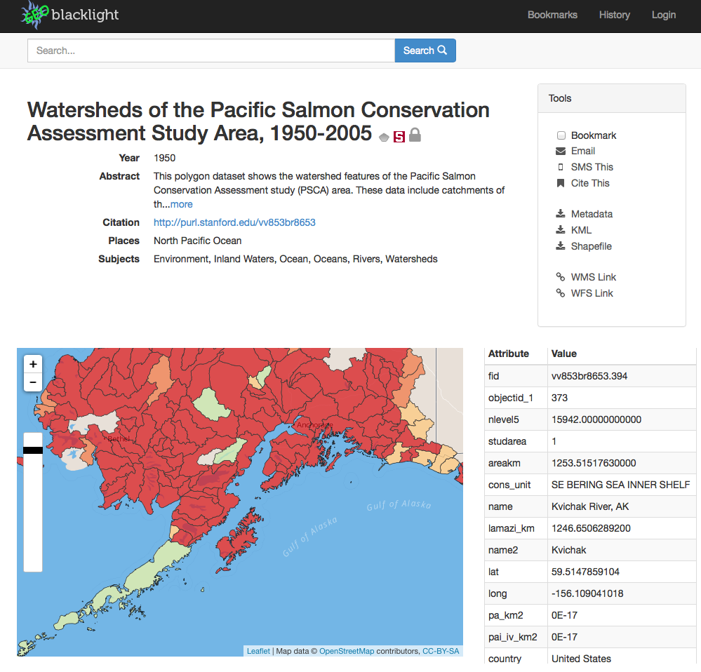
Figure 1. GeoBlacklight prototype of layer view.

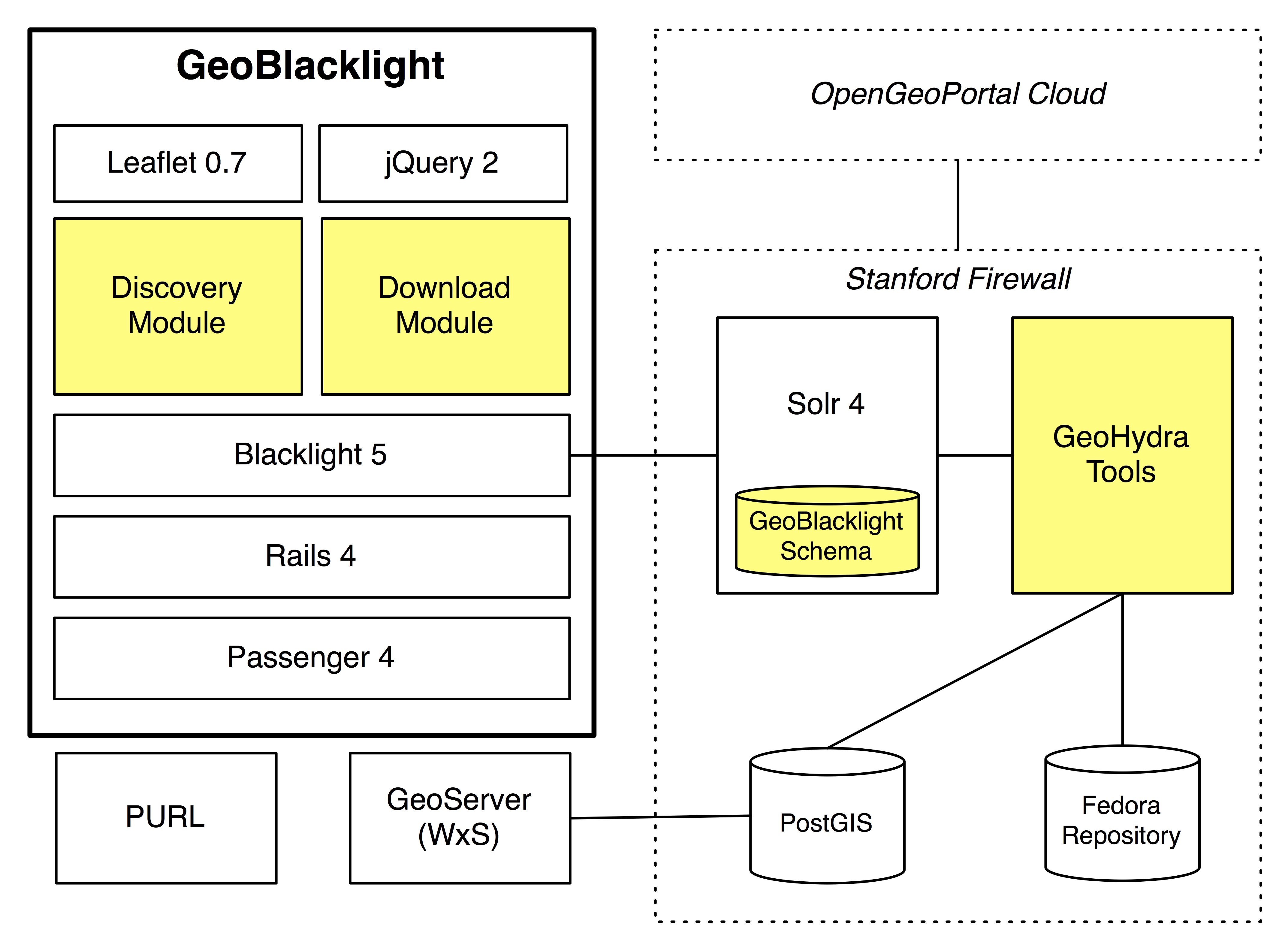
Figure 2. GeoBlacklight’s modular architecture.

Background

GeoBlacklight builds upon prior work on geospatial digital libraries, geoportals, geospatial metadata, and gazetteers.

Geolibraries

A geospatial digital library, or geolibrary, provides an organization and access methods to digital holdings with some geospatial properties. The geospatial properties need not be complex; even point coordinates are useful (Bidney 2010). Goodchild et al. (1999) define a geolibrary as “a digital library filled with geoinformation and for which the primary search mechanism is place.” In the late-90s and 2000s, researchers conceptualized and developed geospatial digital libraries (or “geolibraries”) with various success (Boxall 2003; Erwin & Sweetkind-Singer 2009; Goodchild 2004; Siegel et al. 2004; Smith 1996).

In general, these geolibrary use cases and user interfaces, however, were not geared toward current era search and discovery use cases with natural language inputs and sophisticated relevancy ranking algorithms (Hearst 2009). Instead they were more like electronic catalogs with spatial search as the primary discovery use case (Hill et al. 2000). They also used visualization metaphors from GIS desktop applications, such a multi-layered maps and extensive interactive toolbars. Moreover, these early geolibraries dealt heavily with digital content procurement problems, such as digitization and georectification of paper maps (Westington & Bridge 2013), particularly scaling these methods to large collections.

Geoportals, such as OpenGeoportal, ESRI Geoportal Server [8] and GeoNetwork, [9] are typically “one-stop” shopping applications that focus on discovery of resources within a federated catalog. They are discovery applications that rely on a spatial data infrastructure for delivery and repository services, unlike geolibraries which were more monolithic in nature. Their goal is to provide a destination for domain-specific collections of GIS data (Goodchild et al. 2007). Like geolibraries, they usually do not provide flexible faceted refinement and nagivation of search results, a feature of modern search interfaces (Hearst 2009). They also use similiar user interfaces akin to GIS desktop applications likely due to their underlying assumption of spatially savvy users like GIS professionals, and thus limits their ability to incorporate modern search semantics and visualizations.

Metadata

Metadata that documents the entire lifecycle of a spatial dataset can be extremely granular and may require information regarding data management, data quality reports, or lineage statements that include original source citations and geo-processing activities. While these metadata are important for long-term preservation and subsequent citations, they are often superfluous to the discoverability of GIS resources in a web environment. Moreover, metadata authoring is a labor-intensive process, although research into automated geospatial metadata generation is promising (Hatcheller et al. 2009).

Currently, metadata for geospatial data are created using either the Content Standard for Digital Geospatial Metadata (FGDC) or the ISO Standards for Geographic Metadata. [10] While the more recent ISO Metadata model offers increased potential for standardizing field entries and enables wider adoption among multi-lingual applications, a large store of legacy FGDC metadata exists, documenting several decades’ worth of spatial data production and research (Federal Geographic Data Committee 2014). One of the functions of the GeoBlacklight schema is to reconcile core elements within an aggregation of FGDC and ISO records and to distill them into a set of common search indices.

FGDC or ISO level metadata are considered essential to spatial data infrastructures in order to satisfy the needs of archival and preservation use cases. Creation of source metadata that conforms to either spatial standard is widely recognized as a very time-consuming and labor-intensive process. To alleviate some of these complexities, Stanford has implemented auto-generation for unique identifier elements, and developed batch-editing techniques that expedite the metadata creation process. Additionally, we have created a set of XSLT stylesheets that automatically transform the source spatial metadata into other formats for use in a variety of applications. [11] Therefore, the integrity of the source spatial metadata plays a major role in the quality of discovery metadata that is auto-generated for use in the GeoBlacklight application.

On an international level, attempts to streamline and standardize metadata creation are being addressed by the OpenGeoPortal Metadata Working Group, a multi-institutional partnership of data and metadata experts, who are seeking to develop a set of common community practices for creating and exchanging geospatial metadata. [12] Included in these best practices are recommendations for the use of keyword and name vocabularies, outlining encoding standards for the construction of free-text fields, and methodologies for documenting and relating collection-level metadata to individual layers. This group has been successful in providing guidance for the use and interoperability of the FGDC and ISO metadata standards. A major objective of this partnership is to bring about more normalized and automated methods for the exchange of spatial metadata to ease the burden on local institutional repositories.

Currently, there are several tools available that support the creation of metadata in accordance with either the FGDC or ISO standards. Many of these tools, however, are lacking in one or more fundamental features and often require human intervention in order to fully document and preserve the data. For instance, many institutions maintain licenses for the ESRI mapping software, making the ArcCatalog tool an obvious starting point for metadata creation activity. ArcCatalog provides support for the creation of ISO 19115/19139 metadata, but it does not natively support the creation of ISO 19110 Feature Catalog metadata. The 19110 standard describes data attributes, attribute definitions, and definition sources, metadata that are often considered crucial to using and interpreting data. As a result, Stanford has developed an external XSLT that builds an ISO 19110 record from the ArcGIS formatted metadata.

Gazetteers

Finally, gazetteers are authoritative registries of place names, often with spatial footprints and feature descriptions (Hill et al. 1999). In discovery use cases, users wish to search and browse by location, and gazetteers enable categorical use of place names relative to geospatial location. Increasingly gazetteer services, such as the open-source, community-editable GeoNames, [13] provide linked data interfaces into the place name registry. These interfaces enable new types of discovery uses, such as hierarchical spatial browsing, similarity search, and ontological queries (Kessler et al. 2010). For digital libraries, Freeland et al. (2008) geocoded the Library of Congress Subject Headings (LCSH), but little research has been done to use linked data to integrate the LCSH controlled vocabulary with an authoritative gazetteer. In our prototype, we’ve created a mapping for hundreds of placenames to both GeoNames and LCSH.

Discovery Use Cases

In GeoBlacklight, we focus on discovery-oriented use cases, which are divided into search, view, and curation. The search use cases include three modalities of text search, faceted refinement, and spatial search, and two actors: a casual user and a portal user. On the curation side, there are two actors: a curator and an administrator. Each schema design element, discussed in the next section, enables one or more of these use cases.

Search

Search users either use web search engines or geoportal search directly (Figure 3). This is a very important design point as web search is so heavily ingrained into users’ workflows for discovery of resources in general (Hearst 2009). Thus, the Search use cases include both web search and portal-specific search features of text search, faceted refinement, and spatial search. The result sets are brief and return quickly, and are cleanly organized with title, snippet, institution, and data type. Furthermore, the result sets contain layers from many different institutions as part of a federated multi-institution repository. When the result set layers are clicked, they have a landing page of the layer view use case (Figure 1).

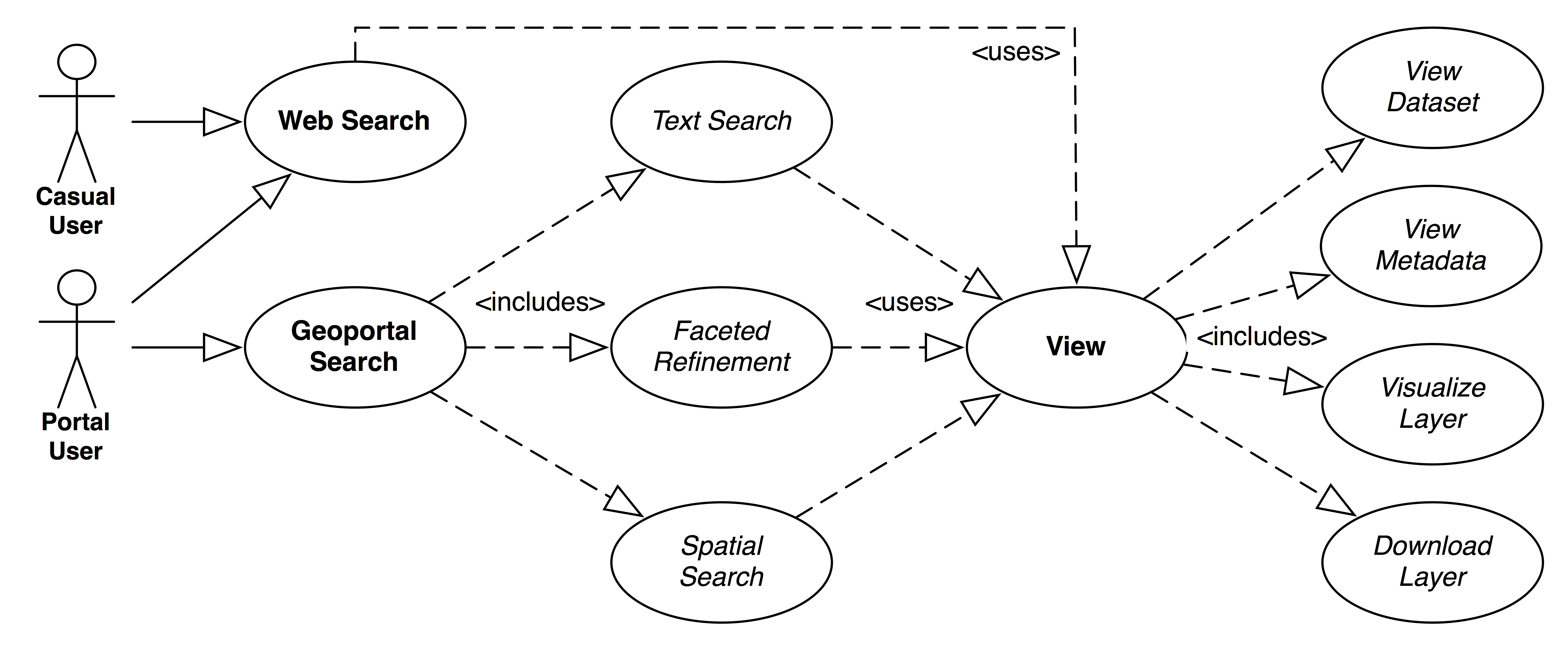
Figure 3. Search and View use cases.

Use case: Web search

Casual users enter in natural language text into a search box of a web search engine. The result sets include layers from the geoportal as well as other relevant results from elsewhere on the web. [14] The result set should show the appropriate title and snippet for the layers. Optionally, the spatial footprint should show on search engines that support spatialized web pages.

Use case: Geoportal text search

Portal users enter natural language text into a search box of the geoportal. This interaction should mimic web search interfaces as users have become accustomed to these simple but powerful interfaces (Hearst 2009).

Use case: Geoportal faceted refinement

Portal users click on categorical facets to narrow their result sets. The facets adjust dynamically to show how many results belong to each facet, and multiple facets can be engaged simultaneously.

Use case: Geoportal spatial search

Portal users zoom and pan a “slippy” web map to narrow their result sets to those results that intersect the current map view. The result set list is ranked by a spatial relevancy algorithm that favors layers with footprints entirely within the current map view. The result list dynamically adjusts as the portal user zooms and pans the slippy map.

View

Both casual and portal users see a view landing page on clickthrough from the result sets. These view pages are shareable, persistent, and bookmarkable via a unique identifier which is important for clear data citation (Michener et al. 2011). They satisfy the following use cases:

Use case: View Dataset

Users view a dataset, which is a collection of individual layers that are related. The dataset has its own descriptive metadata, and a result set with all the matching layers within the dataset.

Use case: View Metadata

Users view the descriptive metadata for either the dataset or an individual layer. The metadata displays with links to appropriate assets such as thumbnail previews or related layers.

Use case: Visualize Layer

Users see a data visualization of the layer within a web map, if available. One issue that affects data visualization with a federated spatial data infrastructure is the latency and reliability of remote data access.[15]

Use case: Download Layer

Users can download the layer data in multiple formats such as GeoTIFF or Shapefile or KML, and then import the data into their GIS desktop application, such as ESRI’s ArcGIS or Google Earth.

Curation

The curation use cases cover how the geoportal application builds and manages its federated multi-institution repository of holdings (Figure 4). These uses cases have two actors: geoportal administrators, and curators (librarians). Administrators ingest remote holdings from many partnered institutions on a regular basis, and they also export their repository’s holdings for other geoportals and web crawlers to ingest. Curators build collections of layers through multiple source channels, such as faculty/student self-deposit, purchasing, and archives public data.

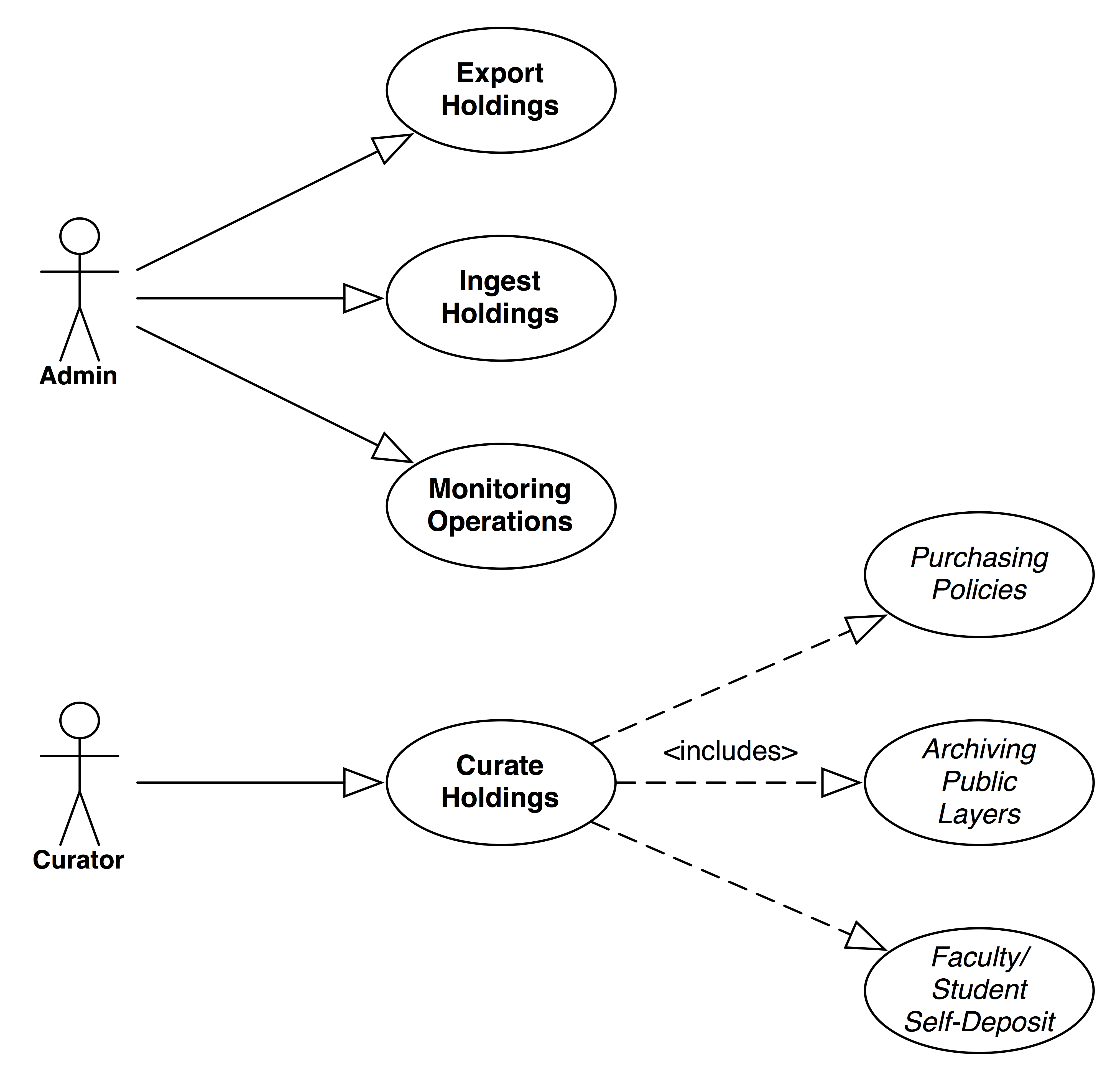
Figure 4. Curation use cases.

Use case: Export holdings

The administrator exports layers from the repository and makes them available to partner institutions to download and ingest into their local geoportal repository. They also export layers to web search engines to enable the web search use case.

Use case: Ingest holdings

The administrator downloads layers from geoportals at partner institutions, and then ingests them into the repository for discovery.

Use case: Monitoring operations

The administrator monitors the operations of the geoportal application and repository to provide a specific level of quality of service.

Use case: Curate holdings

The curator builds collections of layers through multiple source channels, and provides the appropriate metadata for discovery and layer data for visualization.

Use case: Purchasing policies

The curator sets purchasing policies such that newly purchased layers or datasets adhere to metadata standards sufficient for the discovery use cases.

Use case: Archiving public layers

The curator selects and downloads publicly available layer data, such as government holdings for census data. Then, the curator archives the public layers in a repository.

Use case: Faculty/student self-deposit

The curator facilitates self-deposit of layers from faculty and student researchers, and archives these layers in a repository for preservation.

Schema Data Model

The GeoBlacklight schema focuses on the discovery use cases described above. Text search, faceted refinement, and spatial search and relevancy are among the primary features that the schema enables. The schema design supports a variety of discovery applications and GIS data types. We especially wanted to support contextual collection-oriented discovery applications as well as traditional portal applications.

To generate its spatial metadata, Stanford relies on the use of institutional ISO 19139 XML metadata templates to standardize inputs and reduce the number of fields that require manual entry. After the template has been applied and local edits are made to an item’s metadata, Python scripts are run on each record to assign unique identifiers for the data layer, the metadata file, related collection metadata, and feature catalog identifiers (if applicable). Post-scripting, an XSLT processes all records and generates any metadata that is redundant within individual records, such as access URLs or contact details. In some cases, XSLTs are also used as a final step to rapidly perform batch edits on large collections of metadata before they are ingested into the repository.

To achieve a consistent set of metadata elements, the source geographic metadata (ISO or FGDC) are first transformed into the Metadata Object Description Schema (MODS) using an XSLT stylesheet [16] (Figure 5). The resulting MODS is a product of several conversion routines that attempt to normalize the metadata using hardcoded values for genres and resource types, conditional parameters for assigning formats and geometry types, and strict rules for capturing dates or ranges of dates. The MODS schema also supports the use of attributes, including xlink for linking to related concepts or collections, and authority references for topical and geographic subject thesauri (MODS Editorial Committee 2013). The automatic generation of a detailed MODS record also meets the objectives of Stanford’s overall digital library infrastructure by providing metadata for spatial data in a commonly used standard. This allows for GIS objects to be incorporated and searched amongst a comprehensive collection of digital library assets.

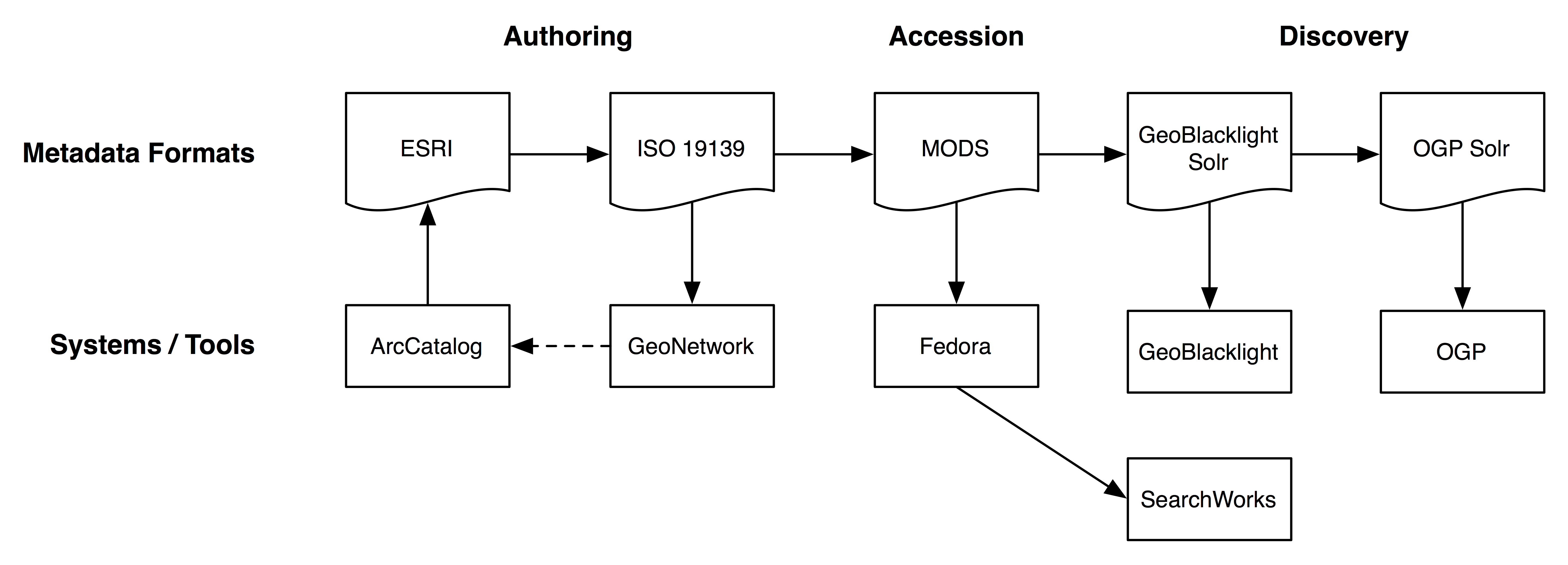
Figure 5. Metadata transformation workflow.

Each layer has a unique identifier stored in the uuid field, noting that each institution may have its own scheme for minting unique identifiers. Dublin Core Metadata Initiative (2011) defines the semantic descriptions of all of these fields. We’re using both DC Elements (dc) and DC Terms (dct). BOLD fields are required, * fields are multivalued.

Term	Description	Example
uuid	Unique identifier	http://purl.stanford.edu/vr593vj7147   http://ark.cdlib.org/ark:/28722/bk0012h535q urn:geodata.tufts.edu:Tufts.CambridgeGrid100_04
dc:identifier	Unique identifier	Often the same as uuid but may be an alternate identifier
dc:title	Title	Digital Map of Village Boundaries of Andhra Pradesh, India, 2001
dc:description	Description	Village boundaries of Andhra Pradesh linked to Census 2001. Includes data for 26041 villages, 237 towns, 23 districts and 1 state. This layer is part of the Village Map of India which includes socio-demographic and economic Census data for 2001 at the Village level.
dc:rights	Rights for access	Restricted, Public
dct:provenance	Source institution	Berkeley, Harvard, MassGIS, MIT, Stanford, Tufts
dct:references	URLs to related services	See Example 1. Uses JSON-LD syntax (http://www.w3.org/TR/json-ld/) with role values based in part on CatInterop (https://github.com/OSGeo/Cat-Interop) link properties.
dc:creator*	Author(s)	George Washington
dc:format	File format of layer data	GeoTIFF, Shapefile
dc:language	Language	English
dc:publisher	Publisher	ML InfoMap
dc:relation*	URLs to related resources	http://sws.geonames.org/1252881/about.rdf
dc:subject*	Subject	Census, Human settlements
dc:type	Resource type	Dataset, Image, PhysicalObject
dct:spatial*	Spatial coverage and place names	Paris, France
dct:temporal*	Years	2010
dct:issued	Date issued	2/18/2008
dct:isPartOf*	Holding dataset	Village Maps of India

For the Dublin Core elements, we use DC:Identifier to implement a unique identifier across a federated multi-institution aggregation of records. We’ve added additional semantics for DCT:Spatial coverage to enable linked data for place names in gazetteers by reconciling text strings and unique identifiers between the GeoNames webservice and the Library of Congress Name and Subject Authorities. DCT:Temporal provides for temporal faceting by date or a range of dates. Similarly, we’ve added additional semantics to DCT:References, reusing a controlled vocabulary from the FOSS4G CatInterop project, [17] which relates content specific to GIS resources, such as Web Mapping Services, and to the original metadata from which the discovery metadata were derived. We use DC:Format with a set of controlled values that are useful for faceting and categorizing existing spatial data types. Finally, we use DCT:isPartOf to relate the resource to a host collection of layers. The schema has a small number of layer-specific elements such as Layer.Slug that enables Permalinks, ensuring all GIS resources are directly addressable via a shareable URL.

We use GeoRSS for geospatial features where only a bounding box element is required. Note that GeoRSS data are in WGS84 (EPSG:4326 projection) and use latitude-longitude (y,x) pairs.

Term	Description	Example
georss:box	Bounding box as maximum values for S W N E	12.6 -119.4 19.9 84.8
georss:point	Point representation for layer as y, x — i.e., centroid	12.6 -119.4
georss:polygon	Shape of the layer as a Polygon in the form S W N W N E S E S W	12.6 -119.4 19.9 -119.4 19.9 84.8 12.6 84.8 12.6 -119.4

The following elements for the discovery application are all layer-specific and all required. These elements have normative semantics specific to the GeoBlacklight application.

Term	Description	Example
layer:id	The complete identifier for the WMS/WFS/WCS layer	druid:vr593vj7147
layer:geom_type	Geometry type for layer data.	Point, Line, Polygon, and Raster
layer:modified	Last modification date for the metadata record	2014-04-30T13:48:51Z
layer:slug	Unique identifier visible to the user, used for Permalinks	stanford-vr593vj7147

Gazetter

The concept of location is fundamental to searching and evaluating spatial data. Metadata in the form of place names helps to contextualize data within a set of coordinates and also provides a method of collocating similar resources based on geographic extent. Current best practices in metadata creation recommend using an existing vocabulary for the identification and assignment of place keywords (MODS Editorial Committee 2013).

For its ISO metadata records, Stanford uses the GeoNames ontology for keyword assignment. GeoNames uniquely identifies geographic entities and provides URIs to concepts and feature documents represented as RDF/XML. The conceptual URIs are embedded into the ISO place keywords XML through the use of the xlink attribute. Although GeoNames identifiers and corresponding URIs are unique, it is often the case that the text strings used to express a place name are not universally unique given the recurrence of place names worldwide. Therefore, it is necessary to construct place keywords using one level of hierarchy (most often the country name), or by addition of an administrative designation (such as ‘District’ or ‘State’), in order to disambiguate between similar entries in the GeoNames database.

Example:
Patiāla (India) – for the city in India
Patiāla (India : District) – for the district in India, which also contains the city

The addition of qualifiers to place names enhances accuracy in the search and retrieval capabilities of the GeoNames database, and also provides a human-readable and unique text string for use in metadata records.

To manage the list of qualified place names, Stanford has developed an open-source gazetteer that establishes links between the GeoNames ontology and the Library of Congress Name (LCNAF) and Subject (LCSH) vocabularies. [18] It is currently created through manual effort. Freeland et al. (2008) implement a similar scheme but use the Google Maps geocoder as an authoritative gazetteer. When parallels exist between the GeoNames and LC ontologies, the gazetteer maps the text string and the unique identifier of the GeoNames entry to the corresponding LC text string and identifier. The qualified version of the place name is also added to the gazetteer record making it available for selection and reuse within other metadata.

Qualified Name	GeoNames Term	GeoNames ID	LC Term	LC Identifier
Patiāla (India)	Patiāla	1260107	Patiāla (India)	n88147583

As a final step, the Library of Congress’ URI is added as a link inside the GeoNames record, permitting users to search for an entry in the GeoNames database using its analogous Library of Congress identifier.

The creation of a linked vocabulary gazetteer allows for the dynamic exchange of place keywords by establishing equivalence among concepts from different ontologies. Since use of the LCNAF and LCSH vocabularies is customary in digital library metadata, the GeoNames data are replaced with their LC equivalents when ISO records are transformed into MODS.

Implementation

Our GeoBlacklight prototype (Figures 1 & 2) uses the Blacklight 5 and Solr 4.7 releases with encodings in both JSON and XML, and metadata standard support for ISO 19115/19139, FGDC, MODS, and the OpenGeoportal Solr schema (Figure 5). The GeoBlacklight Solr implementation is available online at https://github.com/sul-dlss/geoblacklight-schema.

In part, we generate our schema metadata from a MODS record with “geo” extension elements. The MODS specification is vague in how coordinates should be formatted, and in practice there doesn’t seem to be a standard format. The MODS Editorial Committee (2013) writes:

One or more statements may be supplied. If one is supplied, it is a point (i.e., a single location); if two, it is a line; if more than two, it is an n-sided polygon where n=number of coordinates assigned. No three points should be co-linear, and coordinates should be supplied in polygon-traversal order.

We have some internal MODS guidelines at Stanford, but we do not have a normative recommendation for coordinates other than using MARC 034 and MARC 255, both of which have multiple representations. Thus we developed a MODS extension with the following goals:

• Include human- and machine-readable encodings for geospatial coordinates for MODS without requiring a detailed geometries (e.g., paper maps vs. GIS data)
• Clean, simple MODS display logic
• Pass XML validation for MODS 3.4+ schema
• Support point and bounding box coordinates for geospatial indexing, in multiple projections
• Compatible with MARC034 [19] and MARC255 [20] formats. For example, in MARC034 coordinates are encoded as “$dE079.533265 $eE086.216635 $fS012.583377 $gS020.419532”, and in MARC255 they are encoded as “(W 151°28’46”–W 78°5’6″/N 69°25’57”–N 26°4’18”)”.

The human-readable data are in MODS’ subject/cartographics/coordinates element, but the machine-readable data are in a MODS geo extension element which embeds existing geospatial standards. Using the Geography Markup Language (GML) [21] and RDF we can support arbitrary projections for bounding boxes, and using Dublin Core we can define spatial facets like the format (e.g., a Shapefile) and type (e.g., a Dataset with point data), and zero or more associated place names (Figure 6 and Example 2).

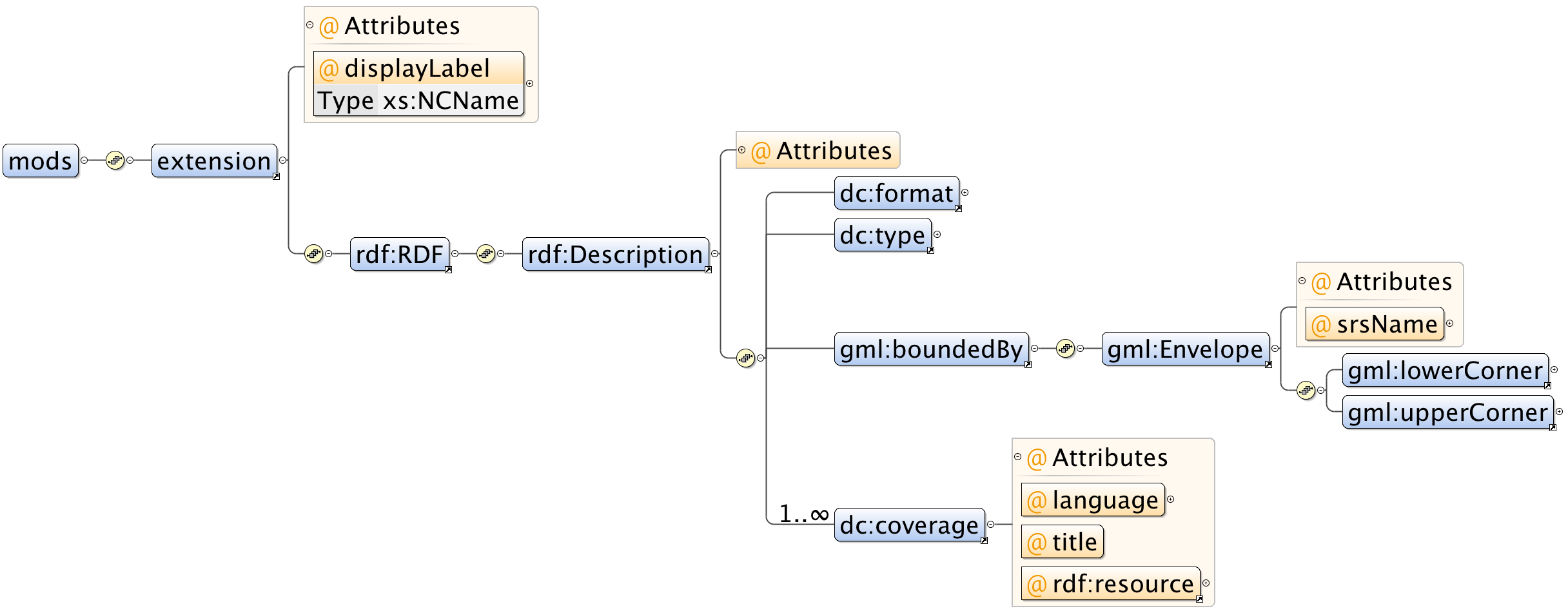
Figure 6. XML schema for MODS “geo” extension.

This is an example of a MODS “geo” extension:

<mods>
  ...
  <titleInfo>
    <title>Oil and Gas Fields in the United States, 2011</title>
  </titleInfo>
  ...
  <subject>
    <cartographics>
      <scale>Scale not given.</scale>
      <projection>North American Datum 1983 (NAD83)</projection>
      <coordinates>(W 151°28?46?--W 78°5'6"/N 69°25'57"--N 26°4'18")</coordinates>
    </cartographics>
  </subject>
  ...
  <!-- RDF encoding for XPath of /mods/extension[@displayLabel='geo'] -->
  <extension displayLabel="geo" xmlns:rdf="http://www.w3.org/1999/02/22-rdf-syntax-ns#">
    <rdf:RDF xmlns:gml="http://www.opengis.net/gml/3.2/"  
             xmlns:dc="http://purl.org/dc/elements/1.1/">
      <rdf:Description rdf:about="http://purl.stanford.edu/cs838pw3418">
        <dc:format>application/x-esri-shapefile</dc:format>
        <dc:type>Dataset#point</dc:type>
        <gml:boundedBy>
          <gml:Envelope gml:srsName="EPSG:4269">
            <gml:lowerCorner>-151.479444 26.071745</gml:lowerCorner>
            <gml:upperCorner>-78.085007 69.4325</gml:upperCorner>
          </gml:Envelope>
        </gml:boundedBy>
        <dc:coverage rdf:resource="http://sws.geonames.org/5332921/about.rdf" 
                     dc:language="eng" dc:title="California"/>
        <dc:coverage rdf:resource="http://sws.geonames.org/6252001/about.rdf" 
                     dc:language="eng" dc:title="United States"/>
      </rdf:Description>
    </rdf:RDF>
  </extension>
</mods>

Using GML, the bounding box can optionally include a valid time period:

<gml:boundedBy>
  <gml:EnvelopeWithTimePeriod gml:srsName="EPSG:4269">
    <gml:lowerCorner>-151.479444 26.071745</gml:lowerCorner>
    <gml:upperCorner>-78.085007 69.4325</gml:upperCorner>
    <gml:beginPosition>2008</gml:beginPosition>
    <gml:endPosition>2008</gml:endPosition>
  </gml:EnvelopeWithTimePeriod>
</gml:boundedBy>

For the Solr 4 implementation, we derive Solr-specific fields solely from other schema properties described in the previous section.

Field	Derived From	Description	Example
solr_pt	georss:point	Point in y,x	12.62,84.76
solr_bbox	georss:box	Bounding box as maximum values for W S E N.	76.76 12.62 84.76 19.91
solr_geom	georss:polygon	Shape of the layer as a ENVELOPE WKT [22] using W E N S.	ENVELOPE(76.76, 84.76, 19.91, 12.62)
solr_jts	georss:polygon	Similar to solr:geom, but using JTS library and POLYGON WKT.	POLYGON((76.76 19.91, 84.76 19.91, 84.76 12.62, 76.76 12.62, 76.76 19.91))
solr_ne_pt	georss:box	North-eastern most point of the bounding box, as (y, x).	83.1,-128.5
solr_sw_pt	georss:box	South-western most point of the bounding box, as (y, x)	81.2,-130.1
solr_issued_dt	dct:issued	Issued date in Solr date format	2001-01-01T00:00:00Z
solr_year_i	dct:temporal	Year for which layer is valid.	2012
solr_wcs_url	dct:references	URL to WCS service	http://example.com/wcs
solr_wfs_url	dct:references	URL to WFS service	http://example.com/wfs
solr_wms_url	dct:references	URL to WMS service	http://example.com/wms

The schema makes heavy use of the dynamicField feature of Solr:

Suffix	Solr data type using dynamicField	Solr fieldType Class
s	String	solr.StrField
sm	String, multivalued	solr.StrField
t	Text, English	solr.TextField
i	Integer	solr.TrieIntField
dt	Date time	solr.TrieDateField
url	URL as a non-indexed String	solr.StrField
bbox	Spatial bounding box, Rectangle as (W, S, E, N)	solr.SpatialRecursivePrefixTreeFieldType
pt	Spatial point as (y,x)	solr.LatLonType
geom	Spatial shape as WKT	Spatial4J version of solr.SpatialRecursivePrefixTreeFieldType
jts	Spatial shape as WKT	JTS [23] version of solr.SpatialRecursivePrefixTreeFieldType

This is an example of the GeoBlacklight schema implementation [24] for the spatial types. Example 3 provides an example document that follows this schema:

<schema name="GeoBlacklight" version="1.5">
  <uniqueKey>uuid</uniqueKey>
  <fields>
    ...
    <dynamicField name="*_d"    type="double"  stored="true"  indexed="true"/>
    ...
    <dynamicField name="*_pt"   type="location"     stored="true" indexed="true"/>
    <dynamicField name="*_bbox" type="location_rpt" stored="true" indexed="true"/>
    <dynamicField name="*_geom" type="location_rpt" stored="true" indexed="true"/>
    <dynamicField name="*_jts"  type="location_jts" stored="true" indexed="true"/>
  </fields>
  <types>
    ...
    <fieldType name="double" class="solr.TrieDoubleField"  precisionStep="8" positionIncrementGap="0"/>
    ...
    <fieldType name="location" class="solr.LatLonType" subFieldSuffix="_d"/>
    <fieldType name="location_rpt" class="solr.SpatialRecursivePrefixTreeFieldType"
               distErrPct="0.025"
               maxDistErr="0.000009"
               units="degrees"
            />
    <fieldType name="location_jts" class="solr.SpatialRecursivePrefixTreeFieldType"
               spatialContextFactory="com.spatial4j.core.context.jts.JtsSpatialContextFactory"
               distErrPct="0.025"
               maxDistErr="0.000009"
               units="degrees"
            />
  </types>
</schema>

The primary query used by GeoBlacklight for spatial search uses polygon containment for spatial relevancy. For example, we issue a Solr query (q) that scores containment by a factor of 10 and uses a text query, then we filter the results (fq) via an intersection spatial predicate:

    q=solr_bbox:"IsWithin(-160 20 -150 30)"^10 railroads
    fq=solr_bbox:"Intersects(-160 20 -150 30)"

The default scoring formula in solrconfig.xml [25] where ^n is the relevancy ranking for the term:

text^1
dc_description_ti^2
dc_creator_tmi^3
dc_publisher_ti^3
dct_isPartOf_tmi^4
dc_subject_tmi^5
dct_spatial_tmi^5
dct_temporal_tmi^5
dc_title_ti^6
dc_rights_ti^7
dct_provenance_ti^8
layer_geom_type_ti^9
layer_slug_ti^10
dc_identifier_ti^10

These fields are all categorical and thus available as facets:

dct_isPartOf_sm
dct_provenance_s
dct_spatial_sm
dc_format_s
dc_language_s
dc_publisher_s
dc_rights_s
dc_subject_sm
layer_geom_type_s
solr_year_i

Conclusion

We describe a metadata schema that enables sophisticated discovery within a geospatial digital library. The schema is designed to support a federated multi-institution repository and facilitates inter-institutional sharing by reusing normative semantics from well-established schemas, Dublin Core and GeoRSS. To reduce duplicate effort we’re also discussing ways to copy catalog for geospatial metadata across partner institutions. Our goal is not only to enable discovery use cases for geospatial resources but also to sizably increase the available resources in the service through easier sharing. We aim to treat GIS assets as durable digital library objects with discovery, delivery, and preservation services.

Acknowledgements

We wish to thank Jack Reed and Bess Sadler for their expertise, work on GeoBlacklight, and comments on earlier drafts. We also thank Amy Hodge and Julie Sweetkind-Singer for their input and discussions about discovery and curation of geospatial resources. We also thank anonymous reviewers for their thoughtful comments. Finally, we wish to thank the GeoBlacklight, OpenGeoportal, and Blacklight open-source communities.

Notes

[1] http://projectblacklight.org
[2] http://opengeoportal.org
[3] http://github.com/sul-dlss/geohydra
[4] http://georss.org
[5] http://projecthydra.org
[6] http://github.com/sul-dlss/geoblacklight
[7] http://lucene.apache.org/solr/
[8] http://github.com/Esri/geoportal-server
[9] http://geonetwork-opensource.org
[10] A series of standards including ISO 19115- the base standard for Geographic Metadata Description, ISO 19139- the XML schema implementation, ISO 19110- the Methodology for Feature Cataloging, and ISO 19119- for describing Web Services.
[11] https://github.com/sul-dlss/geoblacklight-schema/tree/master/lib/xslt
[12] http://opengeoportal.org/working-groups/metadata/
[13] http://geonames.org
[14] DeRidder (2008) provides an example web search integration with a digital library.
[15] https://github.com/sul-dlss/geomonitor
[16] https://github.com/sul-dlss/geoblacklight-schema/blob/master/lib/xslt/iso2mods.xsl
[17] https://github.com/OSGeo/Cat-Interop
[18] https://github.com/sul-dlss/geohydra/blob/master/lib/geohydra/gazetteer.csv
[19] http://www.loc.gov/marc/bibliographic/concise/bd034.html
[20] http://www.loc.gov/marc/bibliographic/bd255.html
[21] http://www.opengeospatial.org/standards/gml
[22] http://spatial4j.github.io/spatial4j/apidocs/com/spatial4j/core/io/WktShapeParser.html. Requires Spatial4J version 0.4, and note the inverted ordering of S and N.
[23] The query performance of the Spatial4J implementation is better than the JTS implementation, in general, due to the more simple spatial predicates in Spatial4J.
[24] https://github.com/sul-dlss/geoblacklight-schema/blob/master/conf/schema.xml
[25] https://github.com/sul-dlss/geoblacklight-schema/blob/master/conf/solrconfig.xml

References

Batcheller JK, Gittings BM, Dunfey RI. 2009. A Method for Automating Geospatial Dataset Metadata. Future Internet 1(1):28-46.

Bidney M. 2010. Can Geographic Coordinates in the Catalog Record Be Useful? Journal of Map & Geography Libraries 6(2):140-150.

Boxall J. 2003. Geolibraries: Geographers, Librarians and Spatial Collaboration. The Canadian Geographer 47(1):18–27.

DeRidder JL. 2008. Googlizing a Digital Library. code4lib (2) [Internet]. Available from http://journal.code4lib.org/articles/43.

Dublin Core Metadata Initiative. 2011. Dublin Core User Guide. Available from http://wiki.dublincore.org/index.php/User_Guide.

Erwin T, Sweetkind-Singer J. 2009. The National Geospatial Digital Archive: A Collaborative Project to Archive Geospatial Data. Journal of Map & Geography Libraries 6(1):6-25.

Federal Geographic Data Committee. 2014. Geospatial Metadata Standards. Available from: http://www.fgdc.gov/metadata/geospatial-metadata-standards#shouldouragencyuseiso.

Freeland C, Kalfatovic M, Paige J, Crozier M. 2008. Geocoding LCSH in the Biodiversity Heritage Library. code4lib (2) [Internet]. Available from http://journal.code4lib.org/articles/52.

Goodchild MF, Adler PS, Buttenfield BP, Kahn RE, Krygiel AJ, Onsrud HJ. 1999. Distributed Geolibraries: Spatial Information Resources. Washington DC: National Academy Press.

Goodchild MF, Fu P, Rich P. 2007. Sharing Geographic Information: An Assessment of the Geospatial One-Stop.
Annals of the Association of American Geographers 97(2):250–266.

Goodchild MF. 2004. The Alexandria Digital Library Project: Review, Assessment, and Prospects. D-Lib 10(5) [Internet].

Hearst MA. 2009. Search User Interfaces. Cambridge: Cambridge University Press.

Hill LL, Frew J, Zheng Q. 1999. Geographic Names: The Implementation of a Gazetteer in a Georeferenced Digital Library. D-Lib 5(1) [Internet]. Available from http://www.dlib.org/dlib/january99/hill/01hill.html.

Hill LL, Carver L, Larsgaard M, Dolin R, Smith TR, Frew J, Rae MA. 2000. Alexandria Digital Library: User Evaluation Studies and System Design. Journal of the American Society for Information Science 51(3):246–259.

Kessler C, Janowicz K, Bishr M. 2009. An Agenda for the Next Generation Gazetteer: Geographic Information Contribution and Retrieval. Seatle, WA: Proceedings of the 17th ACM SIGSPATIAL International Conference on Advances in Geographic Information Systems.

Michener W, Vieglais D, Vision T, Kunze J, Cruse P, Janée G. 2011. DataONE: Data Observation Network for Earth: Preserving Data and Enabling Innovation in the Biological and Environmental Sciences. D-Lib 17(1-2).

MODS Editorial Committee. 2013. MODS User Guidelines (Version 3). Washington DC: Library of Congress. Available from http://www.loc.gov/standards/mods/userguide/index.html.

Siegel D, Burns B, Strawn T. 2004. HGL: A Web-Enabled Geospatial Digital Library. San Diego, CA: Proceedings ESRI International User Conference. Available from http://gis.esri.com/library/userconf/proc04/docs/pap1024.pdf.

Smith TR. 1996. A Digital Library for Geographically Referenced Materials. IEEE Computer 29(5):54-60.

Westington MA, Bridge K. 2013. The Value of a Bounding Box: Moving Historical Charts beyond the Image Browser. Journal of Map & Geography Libraries 9(1-2):108-127.

Examples

Example 1: DCT:References with service URLs

DCT:References = { 
  "http://www.opengis.net/def/serviceType/ogc/wms":"http://geowebservices-restricted.stanford.edu/geoserver/wms",
  "http://www.opengis.net/def/serviceType/ogc/wfs":"http://geowebservices-restricted.stanford.edu/geoserver/wfs",
  "http://www.opengis.net/def/serviceType/ogc/wcs":"http://geowebservices-restricted.stanford.edu/geoserver/wcs",
  "http://www.isotc211.org/schemas/2005/gmd/":"http://purl.stanford.edu/zy658cr1728.iso19139",
  "http://www.loc.gov/mods/v3":"http://purl.stanford.edu/zy658cr1728.mods",
  "http://www.opengis.net/cat/csw/csdgm":"http://purl.stanford.edu/zy658cr1728.fgdc",
  "http://schema.org/url":"http://purl.stanford.edu/zy658cr1728",
  "http://schema.org/thumbnailUrl":"https://stacks.stanford.edu/file/druid:zy658cr1728/preview.jpg",
  "http://schema.org/DownloadAction":"https://stacks.stanford.edu/file/druid:zy658cr1728/data.zip",
  "http://library.stanford.edu/iiif/image-api/1.1/context.json":"http://purl.stanford.edu/zy658cr1728.iiif"
}

Example 2: MODS “geo” extension

<extension displayLabel="geo" xmlns:rdf="http://www.w3.org/1999/02/22-rdf-syntax-ns#">
  <rdf:RDF xmlns:gml="http://www.opengis.net/gml/3.2/" xmlns:dc="http://purl.org/dc/elements/1.1/">
    <rdf:Description rdf:about="http://purl.stanford.edu/dg850pt1796">
      <dc:format>application/x-esri-shapefile</dc:format>
      <dc:type>Dataset#polygon</dc:type>
      <gml:boundedBy>
        <gml:Envelope gml:srsName="EPSG:4326">
          <gml:lowerCorner>68.110092 6.755698</gml:lowerCorner>
          <gml:upperCorner>97.409103 37.050301</gml:upperCorner>
        </gml:Envelope>
      </gml:boundedBy>
      <dc:coverage rdf:resource="http://sws.geonames.org/1252881/about.rdf" dc:language="eng" dc:title="West Bengal"/>
      <dc:coverage rdf:resource="http://sws.geonames.org/1253626/about.rdf" dc:language="eng" dc:title="Uttar Pradesh"/>
      <dc:coverage rdf:resource="http://sws.geonames.org/1254169/about.rdf" dc:language="eng" dc:title="Tripura"/>
      <dc:coverage rdf:resource="http://sws.geonames.org/1256312/about.rdf" dc:language="eng" dc:title="Sikkim"/>
      <dc:coverage rdf:resource="http://sws.geonames.org/1258899/about.rdf" dc:language="eng" dc:title="Rajasthan"/>
      <dc:coverage rdf:resource="http://sws.geonames.org/1259223/about.rdf" dc:language="eng" dc:title="Punjab"/>
      <dc:coverage rdf:resource="http://sws.geonames.org/1260108/about.rdf" dc:language="eng" dc:title="Patiala"/>
      <dc:coverage rdf:resource="http://sws.geonames.org/1263706/about.rdf" dc:language="eng" dc:title="Manipur"/>
      <dc:coverage rdf:resource="http://sws.geonames.org/1264542/about.rdf" dc:language="eng" dc:title="Madhya Pradesh"/>
      <dc:coverage rdf:resource="http://sws.geonames.org/1268731/about.rdf" dc:language="eng" dc:title="Kutch"/>
      <dc:coverage rdf:resource="http://sws.geonames.org/1269320/about.rdf" dc:language="eng" dc:title="Jammu and Kashmir"/>
      <dc:coverage rdf:resource="http://sws.geonames.org/1269750/about.rdf" dc:language="eng" dc:title="India"/>
      <dc:coverage rdf:resource="http://sws.geonames.org/1270101/about.rdf" dc:language="eng" dc:title="Himachal Pradesh"/>
      <dc:coverage rdf:resource="http://sws.geonames.org/1273293/about.rdf" dc:language="eng" dc:title="Delhi"/>
      <dc:coverage rdf:resource="http://sws.geonames.org/1275339/about.rdf" dc:language="eng" dc:title="Bombay"/>
      <dc:coverage rdf:resource="http://sws.geonames.org/1275638/about.rdf" dc:language="eng" dc:title="Bilaspur"/>
      <dc:coverage rdf:resource="http://sws.geonames.org/1275715/about.rdf" dc:language="eng" dc:title="Bihar"/>
      <dc:coverage rdf:resource="http://sws.geonames.org/1278253/about.rdf" dc:language="eng" dc:title="Assam"/>
      <dc:coverage rdf:resource="http://sws.geonames.org/1279160/about.rdf" dc:language="eng" dc:title="Ajmer"/>
    </rdf:Description>
  </rdf:RDF>
</extension>

Example 3: Layer metadata in GeoBlacklight schema

<doc>
  <str name="uuid">http://purl.stanford.edu/zy658cr1728</str>
  <str name="dc_identifier_s">http://purl.stanford.edu/zy658cr1728</str>
  <arr name="dct_isPartOf_sm">
    <str>Village Map of India</str>
  </arr>
  <str name="dc_title_s">Andaman and Nicobar, India: Village Socio-Demographic and Economic Census Data, 2001</str>
  <str name="dc_format_s">Shapefile</str>
  <str name="dc_language_s">English</str>
  <str name="dc_rights_s">Restricted</str>
  <str name="dct_provenance_s">Stanford</str>
  <str name="dc_type_s">Dataset</str>
  <str name="layer_id_s">druid:zy658cr1728</str>
  <str name="layer_slug_s">stanford-zy658cr1728</str>
  <date name="layer_modified_dt">2014-04-17T23:02:53.672Z</date>
  <str name="dct_references_s">{
    "http://schema.org/url":"http://purl.stanford.edu/zy658cr1728",
    "http://schema.org/thumbnailUrl":"http://purl.stanford.edu/zy658cr1728.jpg",
    "http://www.loc.gov/mods/v3":"http://purl.stanford.edu/zy658cr1728.mods",
    "http://www.isotc211.org/schemas/2005/gmd/":"http://purl.stanford.edu/zy658cr1728.iso19139",
    "http://www.opengis.net/def/serviceType/ogc/wms":"http://geowebservices-restricted.stanford.edu/geoserver/wms",
    "http://www.opengis.net/def/serviceType/ogc/wfs":"http://geowebservices-restricted.stanford.edu/geoserver/wfs",
    "http://www.opengis.net/def/serviceType/ogc/wcs":"http://geowebservices-restricted.stanford.edu/geoserver/wcs"
  }</str>
  <str name="dct_issued_s">2013</str>
  <arr name="dct_temporal_sm">
    <str>2001</str>
  </arr>
  <int name="solr_year_i">2001</int>
  <str name="layer_geom_type_s">Point</str>
  <str name="dc_publisher_s">ML InfoMap (Firm)</str>
  <arr name="dc_creator_sm">
    <str>ML InfoMap (Firm)</str>
  </arr>
  <str name="dc_description_s">This point dataset shows village locations with socio-demographic and economic Census data for 2001 for the Union Territory of Andaman and Nicobar Islands, India linked to the 2001 Census. Includes village socio-demographic and economic Census attribute data such as total population, population by sex, household, literacy and illiteracy rates, and employment by industry. This layer is part of the VillageMap dataset which includes socio-demographic and economic Census data for 2001 at the village level for all the states of India. This data layer is sourced from secondary government sources, chiefly Survey of India, Census of India, Election Commission, etc. This map Includes data for 547 villages, 3 towns, 2 districts, and 1 union territory.This dataset is intended for researchers, students, and policy makers for reference and mapping purposes, and may be used for village level demographic analysis within basic applications to support graphical overlays and analysis with other spatial data.</str>
  <arr name="dc_subject_sm">
    <str>Human settlements</str>
    <str>Villages</str>
    <str>Census</str>
    <str>Demography</str>
    <str>Population</str>
    <str>Sex ratio</str>
    <str>Housing</str>
    <str>Labor supply</str>
    <str>Caste</str>
    <str>Literacy</str>
    <str>Society</str>
    <str>Location</str>
  </arr>
  <arr name="dct_spatial_sm">
    <str>Andaman and Nicobar Islands</str>
    <str>Andaman</str>
    <str>Nicobar</str>
    <str>Car Nicobar Island</str>
    <str>Port Blair</str>
    <str>Indira Point</str>
    <str>Diglipur</str>
    <str>Nancowry Island</str>
    <str>Andaman and Nicobar Islands (India)</str>
    <str>Andaman Islands (India)</str>
    <str>Nicobar Islands (India)</str>
    <str>Car Nicobar Island (India)</str>
    <str>Port Blair (India)</str>
    <str>Diglipur (India)</str>
  </arr>
  <str name="georss_box_s">6.761581 92.234924 13.637013 94.262535</str>
  <str name="georss_polygon_s">6.761581 92.234924 13.637013 92.234924 13.637013 94.262535 6.761581 94.262535 6.761581 92.234924</str>
  <arr name="dc_relation_sm">
    <str>http://sws.geonames.org/1278647/about.rdf</str>
    <str>http://sws.geonames.org/1278648/about.rdf</str>
    <str>http://sws.geonames.org/1261448/about.rdf</str>
    <str>http://sws.geonames.org/1274969/about.rdf</str>
    <str>http://sws.geonames.org/1259385/about.rdf</str>
    <str>http://sws.geonames.org/1259116/about.rdf</str>
    <str>http://sws.geonames.org/1272607/about.rdf</str>
    <str>http://sws.geonames.org/1261993/about.rdf</str>
  </arr>
  <str name="solr_geom">ENVELOPE(92.234924, 94.262535, 13.637013, 6.761581)</str>
  <str name="solr_bbox">92.234924 6.761581 94.262535 13.637013</str>
  <double name="solr_sw_pt_0_d">6.761581</double>
  <double name="solr_sw_pt_1_d">92.234924</double>
  <str name="solr_sw_pt">6.761581,92.234924</str>
  <double name="solr_ne_pt_0_d">13.637013</double>
  <double name="solr_ne_pt_1_d">94.262535</double>
  <str name="solr_ne_pt">13.637013,94.262535</str>
 <str name="solr_wms_url">http://geowebservices-restricted.stanford.edu/geoserver/wms</str>
  <str name="solr_wfs_url">http://geowebservices-restricted.stanford.edu/geoserver/wfs</str>
  <str name="solr_wcs_url">http://geowebservices-restricted.stanford.edu/geoserver/wcs</str>
  <long name="_version_">1465674129654939648</long>
  <date name="timestamp">2014-04-17T23:02:53.672Z</date>
  <float name="score">1.0</float>
</doc>

About the Authors

Darren Hardy is a GIS Software Engineer at Stanford University, where he develops open-source geospatial digital library software and services. He earned Ph.D. and Masters degrees in Environmental Science and Management from the University of California, Santa Barbara, and B.S. and M.S. degrees in Computer Science from the University of Colorado at Boulder.

Kim Durante is a Metadata Analyst for Geographic and Scientific Data at Stanford University. She holds a M.S. degree in Information Science from the University of Wisconsin at Milwaukee, and a M.A. degree in Art History from Georgia State University.