by Monica Maceli
Introduction
Text mining has become a popular approach to analyzing and understanding large datasets not amenable to traditional qualitative research techniques. These tools have been applied to a range of information problems, such as understanding themes in social media or facilitating information retrieval in unstructured data. Text mining can be a highly useful tool in the beginnings of research exploration, allowing the textual data to suggest themes and concepts to the researcher during analysis. This can provide a useful starting point for framing further research questions and analysis approaches, particularly if hypotheses and questions are not known in advance (as is typical with an inductive research approach). Furthermore, these tools can also assist in cleaning and structuring text-based data for future analysis in visualization or other graphical tools. And, in addition to the tangible research benefits, text mining can be a fun and fruitful process of discovery!
R is both a language and environment oriented towards statistical computing and graphics creation (R Core Team, 2016). R is made available under the GNU General Public License; as a result of strong community involvement, there have been numerous extensions, called packages, developed over time, as well as robust documentation. Due to this extensibility and versatility, R has remained consistently popular for data and text mining applications across many domains, and includes powerful text mining tools (Meyer, Hornik, and Fienerer, 2008).
The following article will discuss the functionality offered by the text mining package in R, assuming little knowledge of the R language and text mining generally. Although there are numerous online tutorials and resources in this area, an end-to-end exploration of the common functionalities must still be cobbled together across instructional sources, which can be difficult for novice users. The intention of this article is to cover the primary tools and process, such that readers may dive in with their own text collections immediately. Those with pre-existing R experience may wish to skip the following “Getting Set Up” section and proceed directly to the following section on “Working with the corpus”.
Getting Set Up
RStudio[1] is a popular and efficient integrated development environment for working with R, particularly useful for those beginning their work with the R language. In addition to the basic console, many tools are provided in the graphical user interface, including those for: plotting, viewing command history, code completion, and workspace management, e.g. viewing variables currently held in memory. These features, available in the open source and cross-platform version of the tool, can greatly reduce the learning curve; RStudio will be used throughout this article, although the R commands used may be run through any R interpreter.
Precompiled binary versions of R for various operating systems are available at https://cran.rstudio.com/. Upon download and installation of R, the appropriate version of RStudio can then be acquired and installed from https://www.rstudio.com/products/rstudio/download/. The core interaction space in RStudio is the console in the lower left quadrant of the screen (Figure 1, below). The command prompt in RStudio is the > symbol, which you will see followed by a blinking cursor. This is where all commands covered in this article should be entered. The lower right pane of RStudio includes several tabs (one of which provides the R manual). This pane opens by default to the “Plots” tabs in which all graphics, e.g. wordclouds, will appear upon creation.
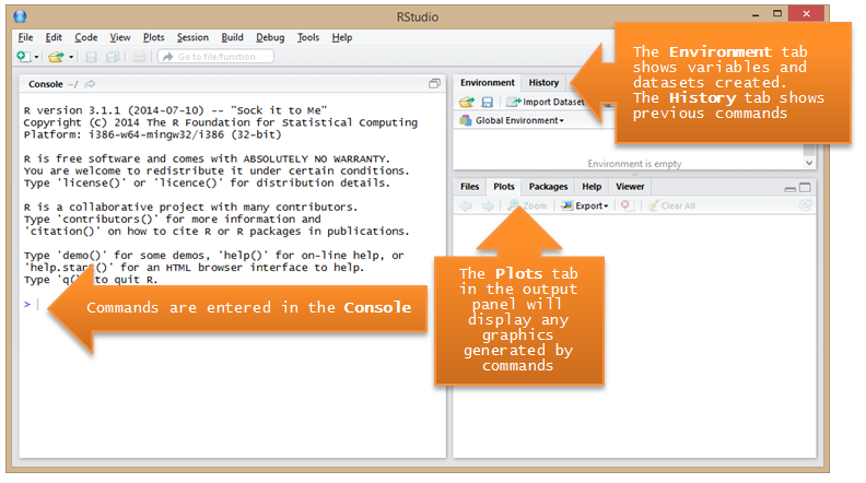
Figure 1. RStudio user interface
If you enter your command across multiple lines, i.e. add a newline within your code, the command prompt will automatically change to the + symbol while you are completing the command. There are many invaluable features[2] in the console that will be familiar to those with command-line experience, including recalling previous commands with the up arrow, and tab completion.
Installing Packages
The base R package includes many useful mathematical and statistical functions. However, for text mining (and later on – wordclouds) we will need to install additional packages. R packages can be installed via the console or in RStudio through the graphical user interface. For text mining, we will use the tm: Text Mining Package (Feinerer and Hornik, 2015) which can be installed by entering the following command in the console or using the “Install Packages” feature in the “Tools” dropdown menu in RStudio.
> install.packages("tm")
Working with the Corpus
The tm package is designed to analyze a collection of text documents, known as a corpus. For this article, we will use a collection of 51 scraped course catalogs to determine prominent and related topics in library and information science programs. A similar approach can be used to analyze text data from a variety of sources, such as tweets or spreadsheet column(s), with a few variations on how the data is input. Examples of alternative input data types will follow at the end of this section, which may better meet your particular text mining needs.
After we install the tm package (as covered in the previous section) we must then load it into the current session using the following command, again entered on the command line in the console:
> library(tm)
Then we will use the Corpus() function to create a corpus of all the text documents contained within the specified directory.
> text_corpus <- Corpus(DirSource('C:/Users/Monica/Documents/Course_Catalogs'))
Once we create our text corpus, we can retrieve summary data about our corpus by entering the corpus name:
> text_corpus
<<VCorpus>>
Metadata: corpus specific: 0, document level (indexed): 0
Content: documents: 51
VCorpus refers to a virtual corpus, meaning this data will be stored until we close our session in R[3]. We can view the content of the first document using the following command. This is particularly useful to view before (and during) text cleaning to ensure we are getting the desired results.
> writeLines(as.character(text_corpus[[1]]))
Next, we will clean the text which serves to remove extraneous characters, unwanted words, and excessive whitespace, to ensure that words are tallied correctly. An important text cleaning task is stemming. Stemming reduces common words to their root, such that the tm package can recognize them as equivalent for counting word frequencies[4]. For example, stemming would reduce "librarians" and "librarian" to the common "librarian", allowing both words to be tallied as the same term. Depending on the dataset, stemming may not be desired, as it has the potential to lose subtle meaning between words. It is also common to remove stopwords, which are very frequently used terms ("and", "the", etc.), as their high frequencies can drown out other important words in our analysis.
The tm package includes numerous transformations to make the process of text cleaning quick and efficient. Most commands have self-explanatory names, e.g. the removeNumbers transformation removes all numbers from the text corpus. The following commands will, respectively, strip extraneous whitespace, lowercase all our terms (such that they can be accurately tallied), remove common stop words in English [5], stem terms to their common root, remove numbers, and remove punctuation. Your individual needs may dictate that you exclude some of these. For example, in a corpus where numbers have meaning that you would like to retain, e.g., the term "3d" or other numeric data, you might skip the removeNumbers transformation.
> text_corpus <- tm_map(text_corpus, stripWhitespace)
> text_corpus <- tm_map(text_corpus, content_transformer(tolower))
> text_corpus <- tm_map(text_corpus, removeWords, stopwords("english"))
> text_corpus <- tm_map(text_corpus, stemDocument)
> text_corpus <- tm_map(text_corpus, removeNumbers)
> text_corpus <- tm_map(text_corpus, removePunctuation)
From our cleaned corpus we can then create the document term matrix and view its summary information like so:
> dtm <- DocumentTermMatrix(text_corpus)
> dtm
<<DocumentTermMatrix (documents: 51, terms: 7891)>>
Non-/sparse entries: 35252/367189
Sparsity           : 91%
Maximal term length: 55
Weighting          : term frequency (tf)
Here we can see that the DocumentTermMatrix() function has created a matrix for us, stored in the dtm variable, with the 51 documents as rows and the 7,891 terms as columns. You'll notice that the sparsity percentage is quite high, which is common as there may be a great number of rare terms, misspellings, etc. throughout the documents that appear very infrequently in the corpus. The dim() function is a handy way to view the numbers of rows and columns of our resulting data structure:
> dim(dtm)
[1]   51 7891
This will be useful knowledge as we reduce our matrix a bit to clean extremely sparse terms as well as prepare for techniques such as clustering (to be covered later on in this article). If we want to reduce some of the sparse terms, and further reduce our matrix size, we can experiment with the removeSparseTerms() function[6]. This function takes two arguments: first, our document term matrix, and second, a number representing how sparse we want to allow a term to be. This sparsity measure ranges from 0 to 1, with numbers closer to 1 meaning a term can be more sparse, i.e. less present in the corpus but still included in the matrix. We can remove some of the sparsest terms and store our new document term matrix into a new dtm2 variable. We can then re-run the dim() function to see the effect:
> dtm2 <- removeSparseTerms(dtm, sparse=0.95)
> dim(dtm2)
[1]   51 2511
Notice that our second document term matrix (dtm2) has become quite a bit smaller! However, one of the difficult balances in text analysis is determining whether the infrequent terms are more (or less) valuable to the particular analysis. Depending on the goals of the researcher, there might be more of an interest in exploring the rare terms than the highly common terms. Alternatively, we can specify the length of words we would like, as well as decide whether we want to exclude very common words. So, in this case, I might determine that I am interested in terms that appear in at least 5 documents, i.e. not too rare, but that do not appear in more than 45 of the documents, i.e. not too common, and that I only want words between 4 and 20 characters long:
> dtmr <-DocumentTermMatrix(text_corpus, control=list(wordLengths=c(4, 20), bounds = list(global = c(5,45))))
> dim(dtmr)
[1]   51 1615
Notice that this approach also yields a significantly smaller set of terms, i.e. columns, in our resulting document term matrix. In particular, the word length requires a bit of forethought – if, for example, you were interested in technology terms such as XML, SQL, etc. you'd want to include shorter term lengths in your term document matrix. We will continue on working with our original document term matrix, dtm, for the following commands, but all commands could be run on a matrix reduced in either (or both) of the means described above.
Working with the Document Term Matrix
Now that we have created the document term matrix, there are a number of built-in functions to assist in understanding our corpus. First, term frequency tends to be a useful starting point in understanding what terms dominate (or trail) our corpus. The findFreqTerms() function can be used to assess a particular document term matrix, with the lower bound frequency you desire:
> findFreqTerms(dtm, lowfreq = 200)
In other cases you may wish to create a full list of term frequencies for use in R or to export; this can particularly be useful to work with or chart in other software, like Excel. The following command creates the freq variable with term and frequency columns:
> freq <- sort(colSums(as.matrix(dtm)), decreasing=TRUE)
We can then use the head() and tail() functions to view a number (in this case 50) of the top-most and bottom-most terms, as desired:
> head(freq, 50)
> tail(freq, 50)
This step may also be useful in indicating that further cleaning of your data is necessary and there may be additional stopwords you'd like to exclude in the cleaning process. The process of document term matrix creation tends to be naturally iterative unless the dataset is very clean and concise to begin with (which it rarely is!) Optionally, we can export the frequency list to a csv (that can be read by Excel or other software) using the following command:
> write.csv(freq, file = "frequencies.csv")
R will save your file to the current working directory; you can see what directory this is by running the getwd(), i.e. get working directory, function:
> getwd()
[1] "C:/Users/Monica/Documents"
If you'd like to change the directory location, you can use the setwd(), i.e. set working directory, command:
> setwd("C:/Users/Monica/Desktop")
Determining the most frequent terms can be a useful first step that can be followed by exploring commonly associated terms. The findAssocs() function takes three arguments: 1) the document term matrix, 2) the term to find correlations with, and 3) the correlation limit, expressed as a number between 0 and 1. A correlation limit of 1 would mean that the terms always appear together. The particular correlation limit chosen may be dictated by the purpose of your research and is worth experimenting with at different values. You may use the frequent terms identified above as a starting point or explore terms you have a pre-existing interest in understanding. For example, the following command would allow you to explore terms associated with the word "humanities":
> findAssocs(dtm,term="humanities",0.8)
If you have stemmed your terms in the text cleaning steps above, you'll want to use the stemmed term in your findAssocs() query as that is how R will be storing the term data. So to find terms correlated with the stemmed term "information" you would use the stemmed version "informat":
> findAssocs(dtm,term="informat",0.8)
A common response to this command is the following message:
> numeric(0)
This simply means that no terms met the correlation criteria with that particular term. So you might try relaxing, i.e. lowering, the chosen correlation limit or pick a more frequent term from the frequency list you've identified above. Once a few interesting term correlations have been identified, it can be useful to visually represent term correlations using the plot() function. If you are using RStudio, the plots will appear in the right-hand plots pane, and can be saved as a PDF/image by using the "Export" dropdown. By default the plot() function will default to a handful of randomly chosen terms, with the chosen correlation threshold, e.g.:
> plot(dtm, corThreshold = 0.80)
However, it is usually far more useful to plot the terms correlated with one of particular interest. Instead of letting R randomly pick terms, we can instead pass in a list of terms that is correlated with our particular target term. The following command will use the now-familiar findAssocs() function to retrieve a list of terms and correlation coefficients associated with "humanities", we will then use the name()[7] function to retrieve just the list of terms returned and pass that into the plot() function.
> plot(dtm, terms = names(findAssocs(dtm,term="humanities",0.8)[["humanities"]]), corThreshold = 0.80)
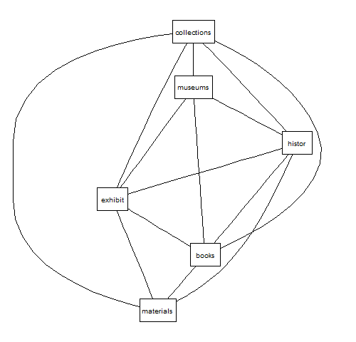
Figure 2. Plot of terms correlated with "humanities"
We can also use the attrs argument to control many of the display characteristics of the plot, e.g. color, node shape, font size, etc. to make it more visually appealing[8].
> plot(dtm, terms = names(findAssocs(dtm,term="humanities",0.8)[["humanities"]]), corThreshold = 0.80, attrs=list(node=list(label="foo", fillcolor="lightgreen", fontsize="16", shape="ellipse"), edge=list(color="cyan"), graph=list(rankdir="LR")))
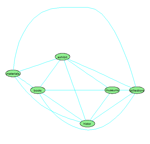
Figure 3. Styled plot of terms correlated with "humanities"
Wordclouds[9] can be another useful visual tool for representing frequencies at a glance. Creating wordclouds in R is quite simple using the Rgraphviz library. We can use our freq variable as created above to pass the terms and frequencies to the wordcloud() function for drawing. First, we will install and load the wordcloud library (which will also load the RColorBrewer package for us automatically), then run the wordcloud() function which takes several arguments: the list of terms, their frequencies, and the minimum frequency term you'd like included. A simple wordcloud can be created like so:
> install.packages("wordcloud")
> library(wordcloud)
> wordcloud(names(freq), freq, min.freq=400)
However, there are many attributes that can be changed to control various aspects of the resulting wordcloud. In the following example, several additions make our wordcloud more visually pleasing.
> wordcloud(names(freq), freq, min.freq=400, max.words=Inf, random.order=FALSE, colors=brewer.pal(8, "Accent"), scale=c(7,.4), rot.per=0)
In order of appearance: the max.words argument controls how many words to plot (in this case, Inf or infinite, meaning all words with greater than 400 frequency); the random.order argument set to FALSE forces the highest frequency terms to be plotted first (and therefore appear in the center of the cloud); and the colors argument, which is commonly used with one of the pre-defined color palettes from the RColorBrewer[10] package[11]. Also available is the scale attribute to determine the size difference between the most and least frequent terms and the rot.per attribute to control how many words are plotted vertically, expressed as a numeric from 0 (all terms horizontal) to 1 (all terms vertical) (Figure 4, below).
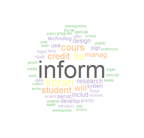
Figure 4. Wordcloud of terms with frequency greater than 400
Lastly, we will explore term clustering. Clustering consists of identifying objects (in our case – terms) that have a similar presence within the documents and grouping them, using a variety of existing clustering algorithms. Clustering techniques are very useful for large corpora where pre-existing categorizations are not known. First, we will create a term document matrix (with terms as rows as opposed to documents), next we'll manipulate the sparsity until we get a nice-size list of terms to work with (usually about 40 terms is the maximum to create a readable cluster size). With this particular dataset, the sparsity percentage needed to be set at 10% to get the number of terms down to a manageable 35. You may want to re-run the removeSparseTerms() function a few times with a different value for sparse=0.1 to get an appropriate number of terms for the particular dataset you are working with:
> tdm <- TermDocumentMatrix(text_corpus)
> tdm2 <- removeSparseTerms(tdm, sparse=0.1)
> dim(tdm2)
[1] 35 51
Next we will shape the data as necessary to run the hclust() function[12] which performs agglomerative hierarchical clustering on our dataset. In this clustering technique, terms are first placed in individual clusters, then the process identifies the nearest (i.e. most similar) cluster and merges the two into a new cluster. This merging process is repeated iteratively until one single cluster is created out of the entire dataset. The following commands will first create a distance matrix representing the similarity between terms, then we will use the hclust() function to apply the clustering technique:
> d <- dist(as.matrix(tdm2))
> hc <- hclust(d)
Lastly, we will use the plot() function to visually display our results in a dendrogram chart (Figure 5, below), which is a tree diagram typically used to graphically represent clusters for ease of analysis.
> plot(hc)
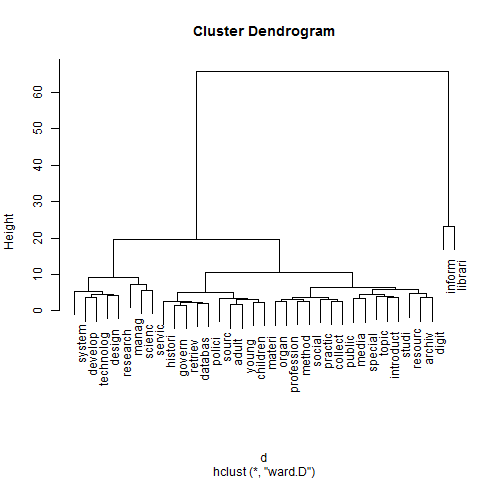
Figure 5. Denogram created through hclust
We can now visually inspect the cluster dendrogram. Interpreting the results of clustering is as much an art as a science. As mentioned earlier, this method of clustering begins by placing each term in its own cluster then evaluating its similarity to other terms; similar terms are then merged into clusters and the process repeats until the clusters are joined into one large cluster. When read from the bottom up, our dendrogram visually represents this step-by-step clustering process that took place. The y-axis of the dendrogram – height – represents the calculated distance between clusters. A small height measure where the terms merge means the distance between terms is small. So the clusters that merged near the bottom of the chart are most similar and tend to co-occur in the documents.
The length of the vertical lines indicates how far apart (dissimilar) the clusters are. We can see that the "inform"/"librari" cluster to the right was not merged until quite high on the chart, meaning that this cluster of terms is quite dissimilar and thus forms a nicely distinct cluster. We are left with what appears to be two distinct clusters – one with "inform" and "librari" and one larger cluster containing all the other terms. We can then use the cutree()[13] function to have R do the work of dividing the "tree" of terms into two clusters and visually outline them on our plot (Figure 6, below):
> groups <- cutree(fit, k=2)
> rect.hclust(fit, k=2, border="red")
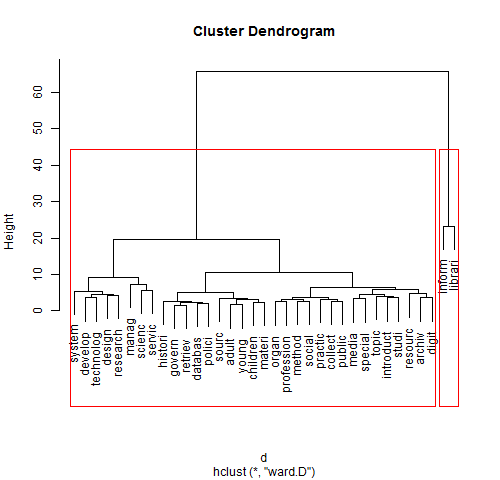
Figure 6. Dendrograms with clusters outlined
Alternatively, in the above commands, we could replace the k=2 with the number of clusters we felt fit the data most appropriately (researchers may interpret a dendrogram differently). A larger and more diverse dataset would likely yield a greater number of distinct clusters than in our example above. Clustering can provide a useful starting point in categorizing documents and understanding the representative terms, particularly to build on what has been gleaned from analyzing term frequencies and correlation.
Other Input Data Formats
We have explored basic text mining commands with a very common use case, working with a corpus consisting of a folder of text documents. Another frequent need is the ability to analyze spreadsheet data. Although R can read in data in Excel formats, it is much easier to work with csv (comma separated value) files. In Excel, the file can be saved as the .csv "Comma Delimited" format (using the "Save As" function), which can then easily be imported into R using the following command. The header argument should be set to TRUE or FALSE depending on whether your data includes a header row:
> text_data <- read.csv("my-csv-file.csv", header = TRUE)
During the next step, creation of the text corpus, instead of the DirSource() function we used with a directory of files, we'll tell R to treat each row of our csv as a distinct document, using the DataFrameSource() function instead:
> text_corpus <- Corpus(DataframeSource(text_data))
The same techniques covered above can then be applied to these alternate data sources: cleaning the text, creating the document term matrix, and then conducting a variety of analysis techniques. These techniques can also be used to shape the data as a series of nodes (the terms) and edges (measure of the closeness of relationships between terms) that can be input to visualization software, such as Gephi[14].
Available Text Data Sources
There are many freely available corpora that can be useful for practicing these text mining techniques, as well as conducting novel research. Browsing these data sources may also spark ideas for mining your own data! As a good starting point, the USC Libraries maintain an excellent research guide listing freely available corpora at http://libguides.usc.edu/textmining/tools, with a mix of full text and metadata offerings. Their research guide notably includes corpora from HathiTrust, Project Gutenberg, Internet Archive, and many others of relevance to the LIS domain. Another very common and increasingly popular use case is mining tweet data retrieved from Twitter's API, using R packages for authenticating and reading Twitter data[15]. No matter the source of the text data, once it is read into R, the same basic commands described above can be used to analyze and interpret the findings.
Conclusion
There is a huge amount of online documentation, tutorials, free courseware, and other online materials dedicated towards learning both novice and advanced tools in R. For those new to the area of text mining in R, this can be overwhelming and require cherry-picking instructions from numerous resources. This article brings together the most common analysis techniques that can be applied to text data, providing an introduction to the powerful text mining functionality available with the tm package.
References
- Feinerer, I and Hornik, K. (2015). tm: Text Mining Package, R package version 0.6-2. Retrieved from http://CRAN.R-project.org/package=tm
- Meyer, D. and Hornik, K. and Feinerer, I. (2008). Text Mining Infrastructure in R. Journal of Statistical Software, 25 (5). pp. 1-54.
- R Core Team. (2016). R: A language and environment for statistical computing. Retrieved from https://www.r-project.org/about.html
Notes
[2] https://support.rstudio.com/hc/en-us/articles/200404846-Working-in-the-Console
[3] Upon closing RStudio, you will be prompted to save your workspace if you wish. This will store your data structures to be reloaded when RStudio is reopened.
[4] The tm packages uses the popular Porter stemming algorithm detailed at http://tartarus.org/martin/PorterStemmer/
[5]You can also create a list of your own stopwords to remove during this step, which is useful if you have words unique to your corpus that you'd like to omit, e.g.:
> my_stopwords <- c(stopwords('english'),'like','learn','use','better','know','etc','id','using','also')
> text_corpus <- tm_map(text_corpus, removeWords, my_stopwords)
[6] http://www.inside-r.org/packages/cran/tm/docs/removeSparseTerms
[7] Note that much existing documentation uses the rownames() function here, e.g.
> plot(dtm, terms = rownames(findAssocs(dtm,term="systems",0.3)), corThreshold = 0.30)
However, this syntax will not work with the latest version of the tm package, as the data structure returned by the findAssocs() function was changed.
[8] The RGraphviz documentation explains the various attributes of the graph that can be controlled in section 4 of https://www.bioconductor.org/packages/devel/bioc/vignettes/Rgraphviz/inst/doc/Rgraphviz.pdf
[9] https://cran.r-project.org/web/packages/wordcloud/wordcloud.pdf
[10] https://cran.r-project.org/web/packages/RColorBrewer/RColorBrewer.pdf
[11] The list of color palettes is viewable by running the command:
> display.brewer.all()
[12] http://www.inside-r.org/r-doc/stats/hclust
[13] https://stat.ethz.ch/R-manual/R-devel/library/stats/html/cutree.html
[15] A concise and illustrated guide to retrieving Twitter data with R is available at https://www.credera.com/blog/business-intelligence/twitter-analytics-using-r-part-1-extract-tweets/
About the Author
Monica Maceli is an Assistant Professor at Pratt Institute School of Information, focusing on emerging technologies in the information and library science domain. She has an industry background in web development and user experience, having held positions in e-commerce, online learning, and academic libraries.

Subscribe to comments: For this article | For all articles
Leave a Reply