by Michael Carlozzi

Background

My public library recently performed a needs assessment as part of its five-year planning process. We distributed a fairly standard patron survey, which asked respondents to evaluate their preferences for and satisfaction with several library-related services. We had also asked survey respondents whether they were interested in joining focus groups.

I had conducted needs assessments before and wanted to do something different this time. So, I performed exploratory factor analysis (EFA) on this survey, as I had speculated that certain “types” of patrons might exist, such as those who preferred quiet study, and that I could identify these types to help improve services. Further, I wanted to recruit patrons who “loaded” on (that is, were similar to) certain factors for our focus groups in an attempt to diversify the candidate pool. In the end, some interesting factors were revealed for future study and analysis, I refined my survey instruments, and we had an engaging focus group which included participants of varied perspectives.

EFA helps researchers to identify latent constructs. Observed data, such as survey responses, are analyzed with the aim of uncovering “factors” that cannot be directly measured. It is a technique which holds broad appeal, used in virtually all disciplines, including library science (e.g., Kwon & Gregory, 2007). And, although factor analysis is mathematically intensive, modern computing means that any practitioner, regardless of mathematical aptitude, can perform it.

This paper is a primer for librarians in the programming language R on using EFA. It hopes to guide interested library workers in conducting such analyses responsibly. While factor analysis is not as inaccessible as it once was, it is still complicated enough that a primer cannot hope to cover all of its nuances and pitfalls. Disagreement exists for virtually all steps of a factor analysis, and due consideration of these options would quickly bog this paper down in technical details. I, therefore, make recommendations based on the work of established researcher Jason Osborne. I would direct readers interested in learning more about EFA to consult Osborne and Anna Costello’s article (2005) and, for a more extensive treatment, Osborne’s book (2014).

EFA simplified; and its uses

Factor analysis is a mathematically complex process which computer programs now fortunately manage. The challenge for human researchers is to perform the analysis responsibly, notably to extract and interpret factors appropriately. Essentially, researchers distribute any item-based questionnaire and then use EFA to determine whether underlying constructs (“factors”) may exist. The payoff is in gaining a richer understanding of phenomenon as well as simplicity; rather than needing twenty questions, for example, to explain something, two factors might instead suffice.

EFA, as the name suggests, is exploratory. Its primary benefit is to help you navigate data in a (hopefully) clear manner based on your preconceptions. That data can take many forms but it is often some type of questionnaire such as a survey. In our case here, you might enter the analysis expecting to find certain “patron profiles,” such as patrons who use the public Internet workstations and not much else. You would hope, then, that an EFA would reveal a factor of those distinct respondents—patrons who showed no real (or even a negative) preference for services outside of public Internet workstations.

But because you are exploring data, firm conclusions should not be drawn. Results should be used to further pursue lines of inquiry or research; other methods, such as confirmatory factor analysis, can analyze structures identified by EFA. Indeed, your goal may not even be to identify the “true” number of factors. In my case, for example, I was more interested in identifying patterns among my users. For example, across four, five, and even six factor models, I was able to notice similar patterns of patron preferences and usage. If one of these models helped clarify these patterns better, then I might choose to settle on that model. Regardless of which model I chose, I was receiving interesting and potentially actionable information about my patron base. So long as you are flexible, do not become married to any particular factor structure, and remain open to the exploration of data/analysis, you should be fine.

Data integrity

Fundamentally EFA analyzes item scales. In other words, it asks how hypothetical factors might “load” onto questions. We can only have faith in analysis if we trust the data on which it has been based. I would recommend, then, using results to refine surveys. The better your survey tools, the clearer your analysis should be.

For example, EFA revealed that my patron survey had several faults. One part of my survey asked patrons to rate their interest on a scale of 1-5 in a particular service. For example, a statement might be “Borrowing physical materials from the library.” It seemed straightforward enough. But I suspect that the survey suffered from a pronounced “halo effect.” In a library setting, the halo effect might occur when survey respondents indicate that they like all aspects of a library’s services because they like the library itself; they therefore have difficulty separating the “parts” (specific services) from the whole. You do not want responses clouded by a halo effect because they will muddle your results.

Indeed, library patrons who fill out surveys usually like the library; in my case, 96% responded that library services overall qualified as “good” or “excellent.” It stands to reason, then, that they would recommend or show interest in services which they did not personally value. In fact, some respondents wrote that, while they did not value a certain service, they rated it highly because they felt it was important to others. I felt obligated to remove those responses, but I have no idea how many users had engaged in similar behavior.

We also had a major problem with respondents who almost exclusively used our English as a Second Language instruction. Despite affirming that they only used the ESOL classes, these patrons almost universally rated highly all library services. As I found this likely the result of a halo effect, I felt forced to remove their responses from the analysis.

Based on these concerns, I suspect that my statement wording was problematic. For future surveys, I plan to design similar questions/statements that instead are more substantive, such as “I wish the library had more dedicated quiet study or reading space.” That kind of user-centered question asks users to rate how valuable quiet study space is to them in a way that (hopefully) distances the response from the library itself, making it (again hopefully) less likely that users will feel a low rating reflects badly on the library.

So, one immediate benefit of an EFA is that it will help you to refine your survey/tests. This, of course, is not limited to EFA, as any comprehensive analysis will achieve the same goal, but factor structures help to reveal readily problematic items/questions.

Now, after you have distributed an excellent survey, you should make sure that your data are structured to facilitate EFA. For best results, collect a lot of responses, analyze only items on the same measurement scale (e.g., all responses range from 1-7 or 1-5), and drop responses with missing data (or fill in those responses consistently; e.g., someone who does not answer a response asking whether he/she liked a service could reasonably be interpreted as not liking that service). EFA needs a large sample. Osborne (2014) recommends a ratio of at least 20 respondents per item; for instance, a survey of 10 items would require at least 200 respondents. Therefore, ensure that whatever data you collect, survey or otherwise, is promoted vigorously and long enough for an adequate sample to be collected.

Further, test items which do not yield much discriminating information should probably also be removed. For example, I had one question that asked, on a scale of 1-5, how “good” library services were. As 96% of respondents answered “good” or “excellent” (not terribly surprising in a survey of active library users), this question failed to discriminate among respondents, so I dropped it.

Installing the necessities

R is a programming language that (almost) trivializes factor analysis. This paper is not a tutorial on R, but the commands presented are simple enough that even total beginners should be able to follow along.

First, you must install the R language. I recommend installing the free and open-source R Studio (www.rstudio.com) IDE/GUI.

One of R’s strengths is the extensibility of its packaging system. R packages contain prebuilt functions that facilitate ease of use, meaning that you do not have to write your own functions. Only one package needs to be installed for this tutorial, “psych.”

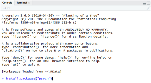
So, once R and R Studio have been installed, run the following command in R Studio to install the psych package. Commands should be run in the Console section, which by default is in the lower-left quadrant of the screen.

install.packages("psych")

After installation, the package must then be loaded. Type the following command:

library(psych)

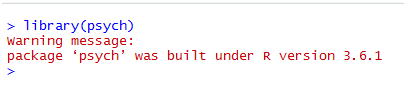
This is not an important warning message; it is not uncommon in R to receive such messages, and in many cases they can be safely ignored.

Loading your data

Your data should be saved as a .csv file as a wide-format spreadsheet (rows for responses; columns for each question on a survey).

The R command getwd() will inform you of the current working directory. Your files must be in the current working directory for R to access them. It is easier to just move your .csv file to that directory than to change the working directory through R’s interface. So, for example, if R tells you that the current working directory is C:/Users/Michael/Documents, move your .csv file to C:/Users/Michael/Documents. It can now be read by R.

After your file sits in the current working directory, you must create a variable of it in R so the program can manipulate it. The following screenshot shows several lines of code which will be explained in turn:

library(psych)
factor_data <- read.csv("factor_cleaned.csv")
head(factor_data)
KMO(factor_data)
five_factors <- fa(factor_data, nfactors=5, fm="pa", rotate="oblimin",
                   cor="poly")

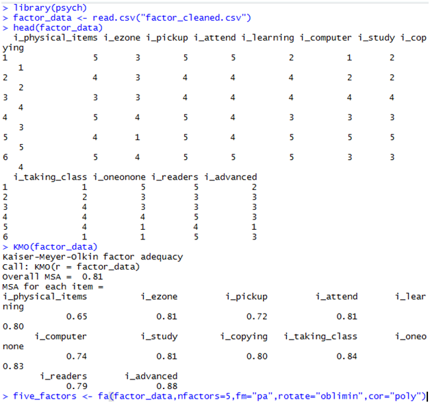
The second line creates a variable called factor_data from the file “factor_cleaned.csv”.  “factor_data” is the name of the R variable and “factor_cleaned.csv” is the name of the spreadsheet with my survey’s responses. In this paper, I have only analyzed data from one part of my survey, the part which assesses patron’s interest (the “i_” of each category) in a service (1 = not interested; 5 = very interested). Each variable is a separate question that the patrons were asked to answer. It is not important to know what all of these variables are now; when necessary, I will explain them.

The command head() returns the first several rows of a data structure. This is a useful command for inspecting how your file’s data have translated to R. If the data look correctly structured, i.e. mirroring your spreadsheet, then you are ready to proceed.

KMO (case sensitive) runs the Kaiser-Meyer-Olkin test. KMO is a quick “sanity check” to ensure that you are not applying factor analysis to inappropriately structured data. Put simply, higher values suggest that the data are amenable to factor analysis. In general, an overall MSA value greater than 0.70 is acceptable. Lower values do not mean factor analysis cannot be done, only that the results should be understood as having wider bands of uncertainty. Individual items with low MSA values may be dropped if, later on, you suspect they are causing problems.

I then run a factor analysis on the final line, storing the results in a variable called five_factors. In this case, I started with five possible factors. The arguments in the command are:

nfactors = the number of factors to extract, in this case 5. It is important to realize that you choose (and experiment with) the number of factors. Indeed, choosing the “right” number of factors is in many ways the most challenging part of EFA. Some techniques exist for helping you choose, which will be covered later.

fm = “pa” is the factoring method, in this case “principal axis factor.” I choose “pa” over maximum likelihood (“ml”) because the data are not multivariate normal (Osborne, 2014, p. 5). To test multivariate normality, install the package MVN (it will also install many dependencies) and refer to the syntax in its help file, (https://cran.r-project.org/web/packages/MVN/vignettes/MVN.pdf). Alternatively, just assume that your survey data are not multivariate normal and default to “pa.”

Readers familiar with some research on factor analysis may wonder whether they can perform principal component analysis (PCA) instead of principal axis factoring. PCA is a popular technique that is often called factor analysis. However, I do not recommend PCA per Osborne (2014), as it is not true factor analysis and is merely a data reduction technique.

rotate = “oblimin” refers to the factor rotation method, which in this case is oblique. Factor rotation helps to “clarify” data structures. There are two primary ways to rotate factors: orthogonal and oblique. Oblique rotations are generally superior and preferred when factors are correlated, which in this case they are (Osborne, 2014). You can probably get away with always using “oblimin” instead of other oblique options (e.g., “promax”) but you can also experiment with other rotation methods to see how they affect the underlying structure.

cor = “poly” is the kind of correlation used, in this case polychoric. This is recommended by van der Eijk and Rose (2015) when analyzing ordinal data, which survey data often are.

The next screenshot depicts output from the factor analysis.

print(five_factors$loadings, digits=2, cutoff=.3)

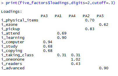
The print command presents the factor loadings (correlations between each factor and survey question) for each factor, generically labeled by the software as PA3, PA1, PA4, PA2, and PA5. Those labels refer to the possible factor chosen. I chose to print only two digits and, arbitrarily, to show only loadings that cutoff at .30. Loadings below .30 were not strong enough to merit my attention.

What essentially happened is that I told the software: please (always pays to be polite) analyze all of the survey responses in a .csv file and build five factors to explain them.

Near 0 loadings/correlations represent no relationship and those with greater values in either direction represent stronger relationships. Note that, when performing oblique rotations, it is possible (but potentially problematic) to have relationships greater than 1.0 (as is the case here with PA4). It is important to remember that loadings close to zero do not represent a negative relationship between the factor and the response, only that the factor is not strongly associated with that response. So, for example, factor PA3 is not strongly associated with interest in borrowing physical items or picking up holds. This does not mean participants who load highly on factor PA3 dislike circulating physical books. That would be the case if they loaded negatively. It means that they are, as a group, no more or less likely to prefer that activity. On the other hand, patrons in PA3 load very highly (0.94) on interest in computing; they are, as a group, far more likely to prefer that activity as well as using the library to study (0.68) and to use the library’s office supply services (0.68).

You’re looking for factors, then, that have clearly defined relationships, that make logical sense (you don’t want, for example, interest in contradictory items), and that do not cross load. Cross loadings mean that items load highly on more than one factor. This is not ideal; in a perfect world, your factors have very little crossover to reflect that they are measuring completely discrete constructs. So, for example, “interest in taking a class” is a bit problematic, because it loads on two factors (both 0.31). One solution may be to remove the item, but since that would omit data it should be a last resort. It makes sense here that an interest in classes would correspond to a factor about general learning (PA1) as well as a factor about one-on-one instruction and eReaders (PA4). Given this logic, I chose to leave the item, planning in future surveys to be more specific about what kinds of classes are being offered.

If you do have lots of cross loadings or a completely unclear structure, then your data may not be suitable for factor analysis. Try writing item questions that more clearly examine different concepts and/or collect more responses. You should also try to adjust the number of factors, as we discuss next.

Wait. How many factors?

Computer programs cannot churn out “the right answers.” It is up to the subject matter expert, here the library staff, to evaluate whether factor structures make theoretical sense. In this way, factor analysis becomes more art than science. There is no magic formula to build, no miracle command to type, which will tell you how many factors are “really” underneath the data. In EFA, you are (predictably) exploring.

I do not recommend, then, following dogmatic prescriptions on selecting the number of factors. Two common but limited approaches recommend choosing factors based on 1) their eigenvalues, the so-called Kaiser criterion, and 2) scree plots. As these are not really recommended methods, I will not detail them. Instead, I prefer to experiment with various numbers of factors and rotation methods to identify something clear, logical, and likely to replicate.

If you would like a more mathematical/computational method, then you probably should use parallel analysis, and, indeed, parallel analysis makes a good starting point. Performing parallel analysis is very easy in R:

fa.parallel(factor_data, fm="pa", fa="fa", n.iter=20, cor="poly")

The command fa.parallel takes an R variable (in this case factor_data) as well as several arguments. The arguments resemble what has been entered before; fm (factoring method) = principal axis factoring, fa = show values for factor analysis, and n.iter = number of iterations to perform, because parallel analysis simulates data. The result of this parallel analysis is why I began with five factors.

However, we should continue exploring to ensure that this solution is the most appropriate.

I now generate a three_factor model, using the same command as earlier to except changing nfactors to 3.

three_factors <- fa(factor_data, nfactors=3, fm="pa", rotate="oblimin",
                    cor="poly")
print(three_factors$loadings, digits=2, cutoff=.3)

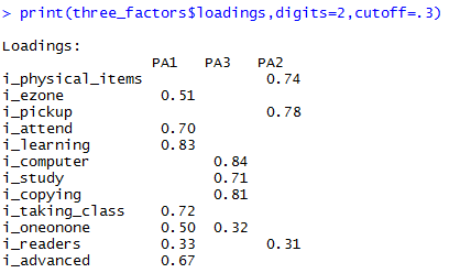
Here, three factors do not really seem sufficient since PA1 loads most questions onto it and we have now two cross loadings. This is not to say the factors are unintelligible. The explanation might be, under this structure, that PA1 represents a default-like patron who likes many library services, that PA3 represents patrons who privilege technology and learning new skills, and that PA2 represents those who really only want to check out items and pickup holds.

four_factors <- fa(factor_data,nfactors=4, fm="pa", rotate="oblimin",
                   cor="poly")
print(four_factors$loadings, digits=2, cutoff=.3)

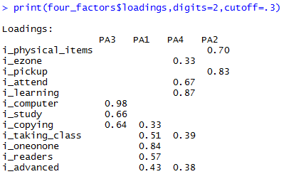
A four factor model, on the other hand, may be a more sensible factor structure; I know of many public library patrons who are mostly interested in isolated and quiet study (PA3). They enter the library without interacting much with staff or other patrons, and consequently show little interest in learning skills from staff. The three factor structured implied that they would have had a modest interest in one-on-one instruction (0.32), which might not be the case.

Five factors, if we recall, also feels plausible. In that structure, we have preserved the isolated users, and we have added a separate group that is interested in learning from library staff (PA4). That one-on-one instruction (1.02) is high alongside eReaders (0.43) suggests that these patrons may enjoy one-on-one eReader instruction. PA5 is now a new factor which represents patrons who are largely interested in eZone, Rhode Island’s electronic book collection (0.62), and advanced technology (0.90). These may be patrons who do not physically come to the library much; indeed, when filtering those respondents who load highly on this factor (see below for factor scores), I find that they are significantly less frequent visitors to the library.

We could consider six factors:

six_factors <- fa(factor_data, nfactors=6, fm="pa", rotate="oblimin",
                  cor="poly")
print(six_factors$loadings, digits=2, cutoff=.3)

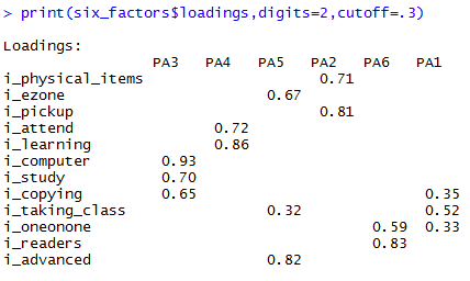
This structure also makes sense, but it suggests that users who like eZone also might want to take classes. This may be true but would merit further investigation.

The five factor model, recommended by parallel analysis, makes a lot of sense, but it has a factor which loads on only two questions; generally you want factors to load on at least three items. On the other hand, the three factor model does not appear to make as much sense. And the others all seem to have positives and negatives.

So, which structure is “correct”? Unfortunately, you can’t tell. One possible way might be to try and replicate certain factor structures across many different environments with confirmatory factor analysis. The structure which replicates best would more likely be the “true structure.” Another way is to attempt to use replication analytics on the current dataset. For example, provided the dataset’s large enough, you might halve it and compare the factors generated in each sample. Osborne (2014) recommends this technique and Beaujean (2014) presents the applicable R code.

Yet all of the factor structures reveal similar service-related patterns. We can fairly confidently assert that some patrons show (group-level) interest in quiet study and solitary space. This pattern emerged in all factor structures. We probably also have patrons who really only seem to care about core borrowing services (holds, physical circulation). This is not to say I will not perform future analyses (I will), but I will proceed as if these patterns do exist. In other words, regardless of which structure is “true,” I have learned something of interest regarding my users.

What’s in a name?

However many factors you settle on, you should name them. Recall our five factor model, where factor PA1 represented patrons who wanted to attend programs (0.69) and learn new skills (0.90). PA1 is not a particularly illuminating name. We might instead label that factor something like the Li(brary)-Curious. I would call PA3 the Invisible Patrons, a term I have used to describe those who come in and use our services but, because they keep to themselves, do not appear on many of our measures; they are, effectively, invisible.

Factor scores

Finally, you can choose to generate factor scores and append those to individual respondents. This is how I was able to recruit specific focus group respondents. Osborne (2014) distrusts factor scores as they are not known for strong replication. He instead recommends more rigorous methods like structural equation modeling. I think, though, that when used with caution and care regression factor scores are OK.

If you would like to generate such scores, then you attach them to the original dataset like so:

factor_data <- cbind(factor_data, five_factors$scores)
write.csv(factor_data, file="new_factordata.csv")

These commands first add factor scores to the original file (factor_data) as another column and then exports that file into a new file (here called new_factordata.csv). Below is a screenshot (edited for clarity) of the new csv file.

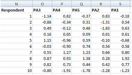
The scores represent how much someone “loads” on a particular factor. Participants who load negatively or positively on all factors should probably be ignored. Ignoring them makes it more likely that you can find someone with clear and definite opinions. For example, respondent 10 loaded (very) negatively on all factors. Reviewing this person’s survey responses, I see that he/she only indicated interest in picking holds up at the library. This also helps me reflect on my survey design, as it suggests he/she did not really understand the statements presented; he/she should have indicated a high interest in physical borrowing as well but did not.

In contrast, respondent 5 loaded highly on PA3 (1.15) and modestly on PA5 (0.59). These factors represent Invisible Patrons (quiet study, computer usage) as well as attending programs and learning new things. Such a respondent appears to want to stick mostly to him/herself but also wants to participate in programs. What kind of programs, for instance, might interest this person?

Limitations of factor analysis; a note on humble expectations

Credible and generalizable research is hard. In this context, one would have to perform an EFA analysis and then perform confirmatory factor analyses, all the while trying to improve both the measurement tools and the library’s services. You shouldn’t expect to receive revelations based on one EFA. As Osborne (2014) emphasizes, “Many researchers use confirmatory language and draw confirmatory conclusions after performing exploratory analyses. This is not appropriate. EFA is a fun and important technique, but it is what it is” (p. 119).

Therefore, results should be interpreted cautiously as they are not necessarily generalizable to other libraries. For instance, readers should not believe that, because my survey had identified what I call Invisible Patrons, that they necessarily exist at other libraries, even those of similar structure (they obviously do, but one EFA cannot determine that). It is also important to understand that locally-designed survey questions are not necessarily reliable or valid measures. Flaws in survey design, many of which I’ve mentioned already in regard to my own survey, introduce uncertainty, clouding results.

Nor should factor loadings be accepted as gospel. Because EFA needs considerable sample size, often at least several hundred participants, significant uncertainty exists around these loadings. I would recommend, then, not interpreting, for example, a factor loading of 0.75 as literally 0.75. Instead, I would suggest that this is a decent-sized loading and reflective of a potentially strong relationship. It is much harder to generate confidence intervals in factor analysis, so I did not cover them here, but make sure that you approach all point estimates with skepticism.

Because of these limitations, I do not think that EFA based on Likert survey data makes for appropriately generalizable research. I think it is best used internally to analyze a particular library’s services. The librarians can refine their analysis as well as their survey instruments to try and identify structures which best approximate their experiences but also offer insights.

In that respect, it bears repeating that the thrust of this article is to help librarians use EFA in R to improve internal services. It is not to argue that the patron types I had identified in our library’s survey generalize to other libraries, public or otherwise.

Conclusion

Despite the aforementioned limitations, I find EFA to be a helpful tool for understanding patron profiles and for improving survey instrumentation. EFA has helped me to not only refine survey instruments but also to consider potentially insightful “patron profiles.” In our needs assessment specifically, it helped me to recruit opinion-diverse focus group participants.

Please remember that this is a very basic introduction to using EFA in R. It should suit most practitioner purposes. Do not hesitate to consult some of the excellent literature on EFA for further information, notably Osborne (2014).

References

Beaujean, A.A. (2014). R syntax to accompany Best practices in exploratory factor analysis (2014) by Jason Osborne. Retrieved from https://www.dropbox.com/s/5cif1thztkodvqf/BestPracticesEFA_Rcode.pdf?dl=0

Costello, A.B., & Osborne, J.W. (2005). Best practices in exploratory factor analysis: Four recommendations for getting the most from your analysis. Practical Assessment, Research & Evaluation 10(7). Retrieved from https://pareonline.net/getvn.asp?v=17&n=15

Kwon, N., & Gregory, V.L. (2007). The effect of librarians’ behavioral performance on user satisfaction in chat reference services. Reference & User Services Quarterly 47(2), 137-148.

Osborne, J.W. (2014). Best practices in exploratory factor analysis. CreateSpace Independent Publishing Platform.

van der Eijk, C., & Rose, J. (2015). Risky business: Factor analysis of survey data — Assessing the probability of incorrect dimensionalisation. PLoS One 10(3). Retrieved from https://www.ncbi.nlm.nih.gov/pmc/articles/PMC4366083/

Appendix

All code in this document:

# installs and loads the required package for the fa function
install.packages(“psych”)
library(psych)                         

# identifies R’s current working directory; must match your
# .csv file location
getwd()

# creates a variable in R of a.csv file
factor_data <- read.csv(“factor_cleaned.csv”)

# displays first several rows of data in variable to make sure
# it loaded correctly from the spreadsheet
head(factor_data)

# performs the Kaiser-Meyer-Olkin test
KMO(factor_data)

# the command below creates a variable in R for a five factor model
# using the arguments factor_data, as the data input, nfactors as the
# number of factors, fm as the factoring method, oblimin as the
# rotation method, and polychoric as the correlation
five_factors <- fa(factor_data, nfactors=5, fm="pa", rotate="oblimin",
                   cor="poly")

# the command below prints to terminal the factor loadings from the
# five_factors variable to two digits, omitting any value below
# (absolute value) of .30
print(five_factors$loadings, digits=2, cutoff=.3)

# changing the number of factors just means changing the nfactors
# argument, as below
four_factors <- fa(factor_data, nfactors=4, fm="pa", rotate="oblimin",
                   cor="poly")
print(four_factors$loadings, digits=2, cutoff=.3)

# the command below performs a parallel analysis on the variable
# factor_data, using pa as the factoring method, factor analysis
# (fa) as the values to show, number of iterations to 20 for the
# simulation, and the correlation = polychoric; the parallel analysis
# recommends the number of factors in the variable factor_data
fa.parallel(factor_data, fm="pa", fa="fa", n.iter=20, cor="poly")

# appends factor scores to the factor_data variable
factor_data <- cbind(factor_data, five_factors$scores)

# creates a new .csv file called new_factordata with the
# new factor_data file (factor scores)
write.csv(factor_data, file="new_factordata.csv")

About the Author

Michael lives and works in Rhode Island. He’s a recovering Joycean and a reluctant instrumentalist.