by Charlie Harper and R. Benjamin Gorham

Using spaCy to Extract Place Names

What Are Named Entities?

A named entity is a “lexical unit referring to a real-world entity in certain specific domains, notably the human, social, political, economic and geographic domains, and which have a name (typically a proper noun or an acronym)” (Novel, Erhman, and Rosset 2016, appendix 5). In practice, named entities include traditional proper nouns, such as person and place names, as well as currencies, dates, named events, and numeric expressions. The definition also extends to field-specific contexts. For example, in medicine, named entities might include genes, pharmaceuticals, chemical compounds, or pathogen names. The extraction of named entities from a text, typically called Named Entity Recognition (NER), can be accomplished with a variety of methods, including regular expressions, statistical models, or neural networks. Numerous Python libraries with pre-built NER capabilities exist. In this article, we employ the spaCy library for NER (https://spacy.io/usage/spacy-101). The spaCy library is free and open source, processes text quickly since it is built into Cython, boasts strong model accuracy, and has a low barrier to entry.

Getting Started with spaCy

After installing spaCy using your package manager of choice (typically with pip install spacy or conda install spacy), you will need to download a language model before you can use the library. As of writing, spaCy has three English language models and additional models for Dutch, German, Greek, French, Italian, Lithuanian, Norwegian, Portuguese, and Spanish, as well as a multilingual model designed to work with mixed texts. The English models come in a small, medium, and large variety, with increasing size, features, and accuracy. We will work with the small English model, which is very lightweight at 11 MB. In contrast, the large model is 746 MB because of added features such as word vectors, which are high-dimensional numerical representations of words. The difference between models, however, is negligible for NER purposes since the NER F-scores, which estimate the model’s accuracy in correctly identifying Named Entities, are comparable, measuring 85.43 and 86.40, respectively.

python -m spacy download en_core_web_sm

To begin using spaCy in Python now requires only two lines of code.

import spacy
nlp = spacy.load('en_core_web_sm')

If you’d like to work with other languages, you can download additional models (see https://spacy.io/models) by substituting the model name for en_core_web_sm in the above download and load syntax.

Processing a Text

By default, a spaCy language model uses a pre-established text processing pipeline (Figure 1) which tokenizes the text (i.e. breaks the text into discrete sentences, words, and punctuation), lemmatizes words (i.e. takes their written form and transforms them to their dictionary entry, such as changing both “writes” and “write” to “write”), tags parts-of-speech, parses syntax dependencies (i.e. how one word connects to another, such as marking an adjective as modifying a particular noun), and labels named entities.

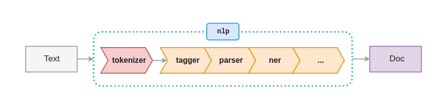
Figure 1. The Default spaCy processing pipeline (from https://spacy.io/usage/processing-pipelines)

Although you can remove parts of this pipeline or add additional components as you see fit, there is immense value in this default behavior; to generate all of this data for a single text, you only need a single call to the spaCy object we created when loading the language model!

import spacy
nlp = spacy.load('en_core_web_sm')

doc = nlp('This is an example of some text to be processed by spaCy.')

The variable doc now holds a spaCy Doc object (https://spacy.io/api/doc) that acts as a container for individual Token objects. The first and easiest way to interact with the processed text is by looping through the document’s tokens and looking at the properties of each. For example, the following will print out each token’s lemma and part-of-speech. Note that the ‘_’ appended to the property names returns a unicode string; without ‘_’ appended to the end of each property, integer values are returned. Each token object has numerous other useful properties and the reader is encouraged to explore these further (https://spacy.io/api/token).

import spacy
nlp = spacy.load('en_core_web_sm')

doc = nlp('This is an example of some text to be processed by spaCy.')

for token in doc:
	print(token.lemma_, token.pos_)

Output:

this DET
be AUX
an DET
example NOUN
of ADP
some DET
text NOUN
to PART
be AUX
process VERB
by ADP
spacy NOUN
. PUNCT

Extracting Place Names

Since we are specifically looking at NER, the Token property ent_type_ is most relevant. If the token is a named entity recognized by spaCy, this property will store the named entity type. Default language models in spaCy currently recognize 18 types (https://spacy.io/api/annotation), two of which refer to spatial entities: GPE and LOC. GPE are geopolitical entities, such as cities, states, and countries. LOC are locations that are not geopolitical entities, such as named bodies of water or forests.

One way to gather all spatial named entities from the doc object is to loop over each token, check its ent_type_, and then build a list of these tokens. Luckily, the spaCy Doc object provides a shortcut that speeds this process up. Rather than looping over every token (many of which will not be named entities), we can use the doc object’s ent property, which is a list of all named entities found in the Doc. Each of these named entities provides the text, the entity type, and the start and end token number (an named entity can be multiple tokens long, such as ‘United States of America’).

import spacy
nlp = spacy.load('en_core_web_sm')

doc = nlp('Ben and I moved to the Cleveland area after school.')

for ent in doc.ents:
	print(ent.text, ent.label_, ent.start, ent.end)

Output:

Ben PERSON 0 1
Cleveland GPE 6 7

Using a list comprehension, we can streamline this to succinctly build a list of all places (GPE and LOC entities) found in a text.

import spacy
nlp = spacy.load('en_core_web_sm')

doc = nlp('Ben and I moved to the Cleveland area after school.')
places = [ent for ent in doc.ents if ent.label_ in ['GPE', 'LOC']]

print(places)

Output:

[Cleveland]

Building a .csv of Place Names in a Corpus

To apply spaCy’s NER to a corpus of texts—in this case, the 500 randomly sampled articles from the CORD-19 dataset—we need to add a bit of code to loop over our texts and then store the results in a single .csv.

import spacy
import pandas as pd
import os

TXT_DIR = 'text'

nlp = spacy.load('en_core_web_sm')
places = []

for fn in os.listdir(TXT_DIR):
    print(f'Processing {fn}')
    with open(f'{TXT_DIR}/{fn}') as f:
        doc = nlp(f.read())
    places.extend([[fn, ent.text, ent.start, ent.end] for ent in doc.ents if ent.label_ in ['GPE', 'LOC']])

df = pd.DataFrame(places, columns=['file', 'place', 'start','end'])
df.to_csv('places.csv', index=False)

This code block is extremely useful. By filling a directory with .txt files, you can quickly generate a .csv of places listed in those files. Moreover, by changing the list of entity labels that the list comprehension uses (currently [‘GPE’, ‘LOC’]), you can actually generate a .csv of any combination of spaCy’s recognized named entities!

Cleaning Place Names and Preparing for Geocoding

If we open ‘places.csv’ and peruse the results, we can see that not everything spaCy has captured is actually a place name, such as “fatigue”, “Appendix S1”, or “d?Pois(?t”. Like all approaches, spaCy’s NER is not perfect and the results require some level of cleaning. There is no foolproof way to remove spurious named entities, but by examining the data we can infer that we might apply a few rules to remove bad places. Namely, those that are all lowercase or contain non-alphabetic characters should be dropped.

import pandas as pd

df = pd.read_csv('places.csv')

def to_drop(place):
    if not all(c.isalpha() or c.isspace() for c in place) or place.islower():
        return True
    else:
        return False

df['to_drop'] = df.place.map(to_drop)

df_cleaned_places = df[df.to_drop==False]
df_cleaned_places.to_csv('cleaned_places.csv', index=False)

unique_places = df_cleaned_places.place.unique()
df_unique_places = pd.DataFrame(unique_places)
df_unique_places.to_csv('unique_places.csv', index=False)

Two .csvs are saved in this code block. After dropping those records that are all lowercase or not alphabetic, a .csv of all cleaned places is saved. Next, to prepare for geocoding the place names, a second .csv of only unique names is saved. This .csv will act as the input for geocoding places and ensures that the same place is not processed and mapped multiple times.

Mapping Place Names with GIS

Once the data has been extracted and sufficiently cleaned, you can then begin the process of transforming it into a geospatial format from a .csv format. In this tutorial, we use ArcGIS software and ArcGIS Online tools in order to generate geospatial data using a process known as geocoding.

What is Geocoding?

Geocoding is a workflow by which cells in a tabular data file are compared to entities with known geospatial locations via a tool called an address locator. The address locator reads the string of each cell in a user-defined selection and scans for matches in a reference dataset. If a match is found, the location data is appended to the input entry and a match score assigned based on the level of confidence that the data in the cell indicates the entity in the address locator. For example, an input cell with the string “123 Main St.” would return a higher match score than a cell with “123 Main” when matching against a reference data entry that reads “123 Main Street.” The geocoding process utilized in the current study employed pre-built tools available in the ArcMap and ArcGIS Online platform, and the steps by which the results were achieved are outlined below.

It is important to note that geocoding a table of addresses with ArcGIS Online, ArcMap, or ArcGIS Pro is not a free service, and consumes credits that can be purchased ad-hoc or as part of an institutional subscription. Pricing is variable by plan, but regardless of how they are obtained, geocoding 100 addresses consumes 4 credits. A full description of credits can be found here: https://doc.arcgis.com/en/arcgis-online/administer/credits.htm

When geocoding a table of locations or addresses via this process, users rely on an address locator to assign geospatial matches to entries in the input table. Address locators are available in a variety of styles, including Single Field, Dual Range, City State Country, and many more.

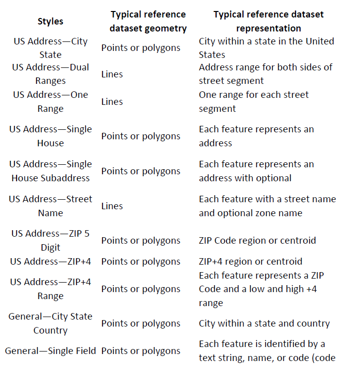
Figure 2. Partial List of Address Locator Styles, adapted from https://desktop.arcgis.com/en/arcmap/10.3/guide-books/geocoding/commonly-used-address-locator-styles.htm

Regardless of the style of address locator, the functional principle of its operation is the same. A collection of reference data forms the structure of the locator, providing a set of features to be matched against. Reference data may consist of point features representing cities, line features representing road segments, or polygons representing administrative boundaries such as census tracts. Each of these features includes string values describing or defining the feature, so a point feature describing Cleveland, OH, may include the fields and values “City or Town: Cleveland,” “State or Province: Ohio,” and “Country: United States of America,” among others to fully describe the feature. The reference data needs to cover the full geospatial extent of the study data. If locations within the input dataset fall outside the scope of the reference data (for example, the reference data consists of line segments representing streets within the continental United States, but the .csv file to be geocoded contains addresses in Canada), the address locator will fail to find matches and will result in gaps in the output.

For the present tutorial, we use the ArcGIS World Geocoding Service, a pre-built service that employs a robust address locator appropriate for finding locations all over the world.

The data scraping and cleaning process described above results in a .csv file with a single field that describes the location of each entity. Such a format is ideal for Single Field address locator styles, but can also be used in other styles that expect (but do not require) multiple field inputs. For many address locators, more precise locational data will be returned if the .csv has multiple fields including street address, street name, city, state or province, country, etc. The address locator will match the string values from these input fields against the full range of entries in its reference dataset and can return multiple matches for each entry. For example, a string value of “100 Main St., Springfield” with no postal, state, or country identifiers will produce multiple potential matches that the user can select from after the geocoding has completed.

The geocoding process in the present tutorial was performed using the ArcGIS Online interface. Two workflows to achieve the same end result will be described below, one using a desktop installation of ArcMap 10.8 and one using the ArcGIS Online interface.

Option 1: Geocoding in ArcMap

To geocode a table of addresses or locations via this method, the user will need the following:

1. A working installation of ArcMap 10.6 or higher.
2. An active internet connection.
3. An ArcGIS Online account with the ability to spend credits.

First, open ArcMap, open a blank map document, and sign into an ArcGIS Online account with access to credits. This can be done via the File menu once the map document has been opened and the machine is connected to the internet.

You may wish to add the Geocoding toolbar to your ArcMap workspace to facilitate access to the geocoding tool. The tool can also be found via the search window (search: Geocoding) or via the ArcToolbox interface (Geocoding Tools). The toolbar can be added to the workspace by navigating to Customize>Toolbars>Geocoding.

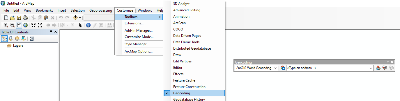
Figure 3. In the Main Menu toolbar, navigating to Customize>Toolbars will show a full list of available toolbars that can be activated for your mapping session.

On the Geocoding toolbar that you have now activated, select the mailbox icon (Geocode Table of Addresses). The tool prompts the user to select an address locator to use, and supplies two default options, the ArcGIS World Geocoding Service or the Military Grid Reference System. You may also add other address locators to the list if they have either created them from reference data or obtained them from other sources, but that is outside the scope of this article. For thorough documentation on building an address locator, see https://desktop.arcgis.com/en/arcmap/latest/manage-data/geocoding/creating-an-address-locator.htm

Figure 4. Clicking on the mailbox opens the address locator selection, and after selecting your address locator you can browse to a locally saved .csv to geocode.

The geocoding interface for the chosen address locator (ArcGIS World Geocoding Service) appears, and the next step is to input the .csv dataset of addresses that is ready to be geocoded. Navigate to the correct file in the “Address Table” input field and choose “Add.” Depending on how the data has been formatted, you can now choose to geocode using a single field or multiple fields. The single field option will read string data from a single column of cells and match each entry against the strings in the corresponding fields of the address locator’s reference data. Single field data can be as simple as the name of a country or city, or it can take the form of full address information with comma-separated values distinguishing between city, country, zip, etc. Choosing multiple field geocoding suggests that the dataset has multiple columns of string values that represent different components of an address. One field stores street addresses, the next stores the name of the city or town, another stores the state or province, etc.

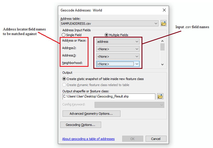
Figure 5. The right column of the geocoder window allows you to specify which field names in you .csv you want to be checked against fields in the address locator. If your .csv does not have a corresponding field for every field in the address locator, those can be left blank.

For single field geocoding, click the dropdown menu and ensure that the location field is selected. For multiple field geocoding, map each of the address locator fields to their corresponding columns in the input .csv file, and leave any unused fields on the “<None>” value.

The geocoding process reads the inputs from the .csv and matches them against the reference data to produce an output shapefile of point features. There are two options for how this output shapefile will be saved: a static file with the .csv data appended to the corresponding geospatial features or a dynamic feature class that includes a “relate” to the data in the .csv file. Relates may always be added later, so we recommend the first option for the sake of simplicity. Choose your preference, specify the name and location of this output shapefile, and run the tool by clicking “OK.”

The tool will display the matching process and record the total number of matched, tied, and unmatched addresses. Tied addresses indicate the address locator found multiple possible matches with the same score, such as “123 Main St” and “123 Main Street.” When the process is complete, you have the option of “rematching” the data to manually correct any unmatched address or clarify any tied addresses if necessary. The resulting output consists of a point shapefile with each feature corresponding to a location from the input .csv file that has been matched with coordinates from the reference dataset of the address locator. You can inspect the feature data by right-clicking the layer in the table of contents and selecting “Attribute Table” to confirm that the locations represented are correct.

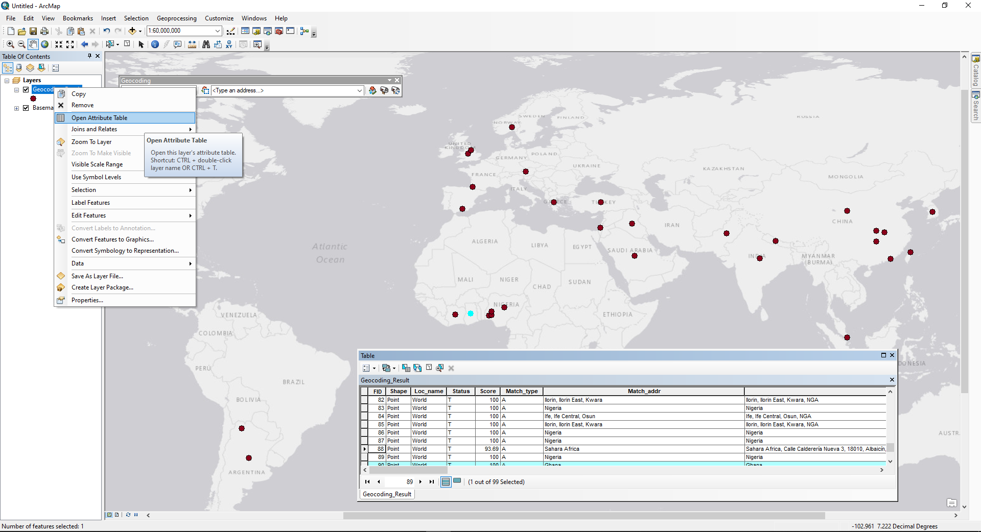
Figure 6. Screenshot of the ArcMap window displaying the geocoded addresses as points on the map. The attribute table for the geocoded list of addresses is accessible by right-clicking the layer.

At this point, the map document can be saved and uploaded to ArcGIS Online as a web map. To create a webmap, you should first save the map document locally as a .mxd file, the default filetype for ArcMap documents. Within the saved document, search for the “MXD to Web Map” tool in the Server>Publishing toolbox. This tool publishes a web map to the user’s ArcGIS Online content with the layers and symbology as it is currently saved in the local ArcMap document. The “MXD to Web Map” tool allows users to specify the name of the output web map (which can differ from the name of the locally-saved .mxd if you want) and requires at least one tag to be attached to assist in categorizing the web map. A brief summary is also required to describe the web map. If the saved .mxd has more than one layer, you can specify which layers you want to appear in the web map, and then click “OK” to publish the web map to your ArcGIS Online content.

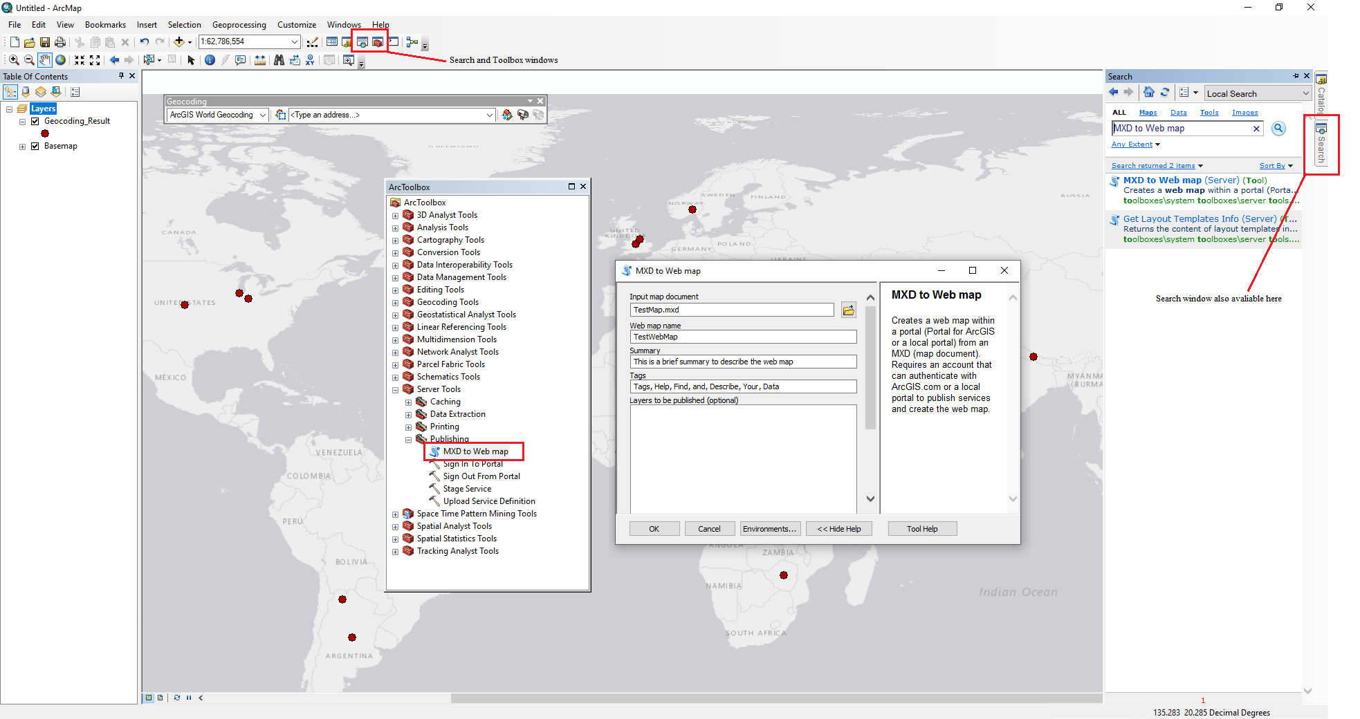
Figure 7. The Search window and ArcToolbox are accessible from the standard toolbar, and will open windows allowing you to explore or search for the full set of tools available in ArcMap. Pictured is the MXD to Web map tool window.

This process results in a web map saved in your arcgis.com content. The next section describes an alternate method to achieve the same result.

Option 2: Geocoding with ArcGIS Online

Another, far less complex method of geocoding a table of addresses is to do so directly on the ArcGIS Online platform. Whereas the previous method involved local installations of software and searching for tools to use, this method simply requires the user to upload the .csv file to an open web map.

To geocode directly in ArcGIS Online, the following are required:

1. An active internet connection.
2. An ArcGIS Online account with the ability to spend credits.

The first step is to sign into your account on arcgis.com. From your arcgis.com home page, click “Map” from the menu at the top to open a blank web map to which the data can be added and geocoded. A blank map will open displaying a default basemap of the world. Content, including the table of addresses to be geocoded, can be added to the map by clicking the “Add” button and selecting “Add Layer from File.” In the “Add Layer from File” dialog, choose “Browse” and navigate to where the .csv file has been saved, and choose to import the layer.

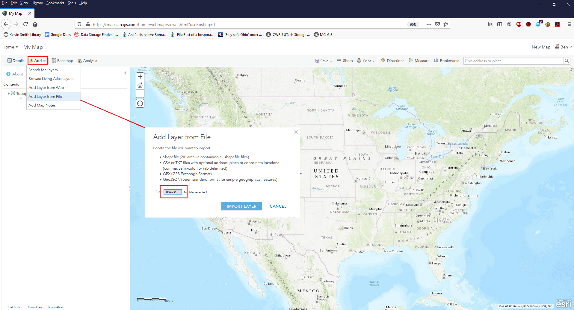
Figure 8. The Map interface on arcgis.com, showing a blank map canvas with default basemap. Data can be added using the Add button at the top left.

The following dialog presents an option of how the .csv file should be imported; as a raw table or as data to be geocoded. Depending on the geographic range of your input data, choose the appropriate coverage in the drop-down menu: we chose “World” to ensure that the input data will be compared to reference data from the entire world. To geocode the locations in the table, choose the “Locate features by” option that corresponds to the format of the locations. If the table uses latitude and longitude, select “Coordinates,” and if the table uses place names or addresses, choose “Addresses or Places.” It is essential to then confirm that the field names in the input .csv file are being correctly mapped to the fields in the reference data. Depending on the format of the data, select each line in the “Location Fields” column and ensure that it matches the field from the input dataset.

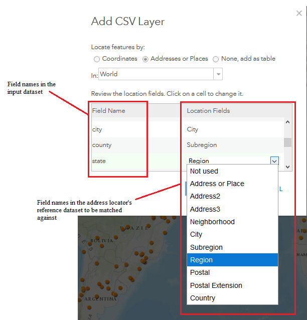
Figure 9. The fields from the locally saved .csv are visible on the left, and the fields they will be compared against are visible on the right. Select a matching field for each of the input fields you wish to use during the geocoding process.

When the fields have been appropriately mapped, click “Add Layer” to run the geocoding process. The entries in the .csv file will be checked against the reference dataset by the address locator based on the selections described in the above paragraph, and an output layer will be generated that displays the geospatial locations of each matched entry. You may now modify the style or symbology of the features in the layer to your preferences; such changes may be made at any point in the future as well. The feature layer also retains the data from the .csv file in its own attribute table, which is viewable and editable in the content pane of the web map by mousing over the layer and clicking “View Attribute Table.”

Linking the Article Data to the Map

Now that the unique places have been geocoded, we can link data on the articles that mention them. In this case, we will upload our cleaned_places.csv and link the article filename to each place. You can go further to link any type of data you’d like, including more detailed metadata on each article.

To upload the cleaned_places.csv, in the top left Home dropdown, click Content. Under the loaded content page, the “Add Item” button will let us upload our .csv from our computer. We’ll title this layer “CORD-19 Articles” and under the “Locate features by” heading, we’ll select “None” since this file has no coordinate data stored within it. Once this upload finishes, we can return to the map and then click “Add -> Search for Layers.” The “CORD-19 Articles” layer will appear and can be added to the map.

Figure 10. The upload screen to add our cleaned_places.csv to ArcGIS Online.

To link this .csv with filenames to places, use the Analysis button along the top toolbar of the map. This opens the Analysis pane, with a variety of options. Under “Summarize Data” click “Join Features.” Our target layer will be the point layer UniquePlaces and the layer to join will be the newly added “CORD-19 Articles.” We’ll choose fields to match and set both fields to place. Use a descriptive title to name the layer. Here, we used “Places to Articles”. The join operation will be one-to-many since one mapped place can join many separated articles. Then click Run Analysis to create the join.

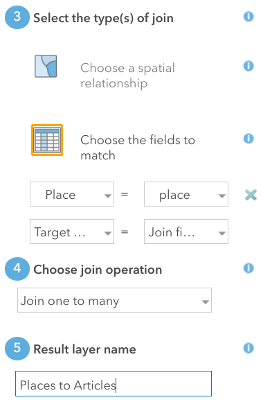
Figure 11. Join Features allows you to link data by place name and visualize this relationship in the map.

With this layer created, all of the data of interest is stored in a single place, and we can remove the previous UniquePlaces and “CORD-19 Articles” layers. Clicking on any point in the map now shows a pop up that lists the number of mentions for that place and provides individual information on the file in which it is mentioned as well as the starting and ending token number. This is also where additional metadata on an article would be displayed if you choose to join it. Iceland, for example, has five appearances in the texts and if this were an area of interest, we could now quickly find out which articles to look in.

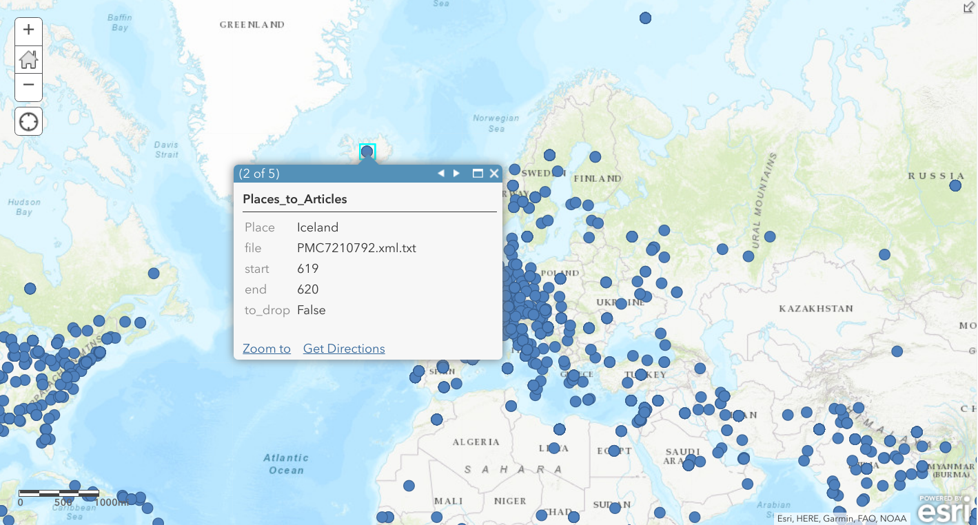
Figure 12. Clicking on a place in the map now shows how many times the place appears in our corpus and the file it appears in.

Finishing Up the Map

By navigating to the Content page, users can view and edit the details of the webmap. The item page for the web map allows the uploader to augment the metadata associated with the file, and provide an in-depth description, tags, credits, and attribution data. Including such metadata will improve the discoverability and citation metrics of the web map, should you choose to make it public. On the web map’s item page, choosing to “Open in Map Viewer” will enable editing the map’s symbology, attribute table, and information pop-ups. Each of these can be adjusted by mousing over the layer in the web map’s table of contents and selecting the corresponding item.

You should now have a functional, customized web map showing the geospatial locations of features from your original .csv file that can display information from its attribute table as a popup. You can edit and save this map to your content on arcgis.com and choose its level of sharing and privacy. You can continue to add data and modify the web map as you see fit and use it to generate web apps from the item description page in your content section of arcgis.com.

Bibliography

Nouvel, D., M. Erhmann, and S. Rosset. 2016. Named Entities for Computational Linguistics. Wiley: Hoboken, NJ.

About the Authors

Charlie Harper is the Digital Scholarship Specialist at Case Western Reserve University, where he collaborates on and manages a variety of digital projects. Much of his work centers on the interdisciplinary applications of machine learning, text analysis, and GIS.

R. Benjamin Gorham is the Research Data and GIS Specialist at Kelvin Smith Library, Case Western Reserve University. With a degree in Classical Archaeology, Ben specializes in the digital humanities with a focus on GIS, photogrammetry, and network analysis and serves as geospatial supervisor for a number of archaeological projects in the Mediterranean. At Case Western, he works with researchers across the university to integrate GIS workflows and technologies towards the advancement of research goals.