by Emily Cukier
Introduction
The General Index (GI) is a massive corpus of text data derived from published articles; its stated purpose is to open scholarly literature to public inquiry. The GI contains tables of keywords [1], ngrams, and associated metadata extracted from a corpus of over 107 million journal articles drawn from general and specialized journals [2]. This enables full-text searching of a wide swath of academic literature in a single shot, without limitation by vendor platform or paywalls.
The GI is the output of a mass journal article accumulation project spearheaded by open information advocate Carl Malamud and conducted at Jawaharlal Nehru University (JNU) in New Delhi [3]. Public Resource, a nonprofit founded by Malamud, released the first public version of the General Index in October 2021 [4]. As of this article’s publication, it contained articles published as recently as 2020.
The GI could be a powerful aid to librarians and digital humanists for tracking concepts through scholarly literature. One clear application is in literature review and systematic searching: one can query search terms simultaneously across more articles and disciplines than contained in even the largest vendor discovery platforms, and without permission to access full text [5]. With minimal manipulation one can link term instances to publication years, enabling diachronic analysis of word usage over time. This allows for visualization of trends in journal articles, much like Google Ngram Viewer does for books. But unlike Google, the GI links keyword and ngram data to the document of origin, which enables identification and retrieval of the works.
A substantial obstacle to using the GI is lack of an exploratory interface. The user must download the raw data tables, then devise methods for querying the records. Even though the tables are split into slices, reading them requires more disk space and memory than found in typical desktop computers.
With some deliberate programming choices and tricks, it is still possible to use portions of the GI in a limited computing environment. This paper will present one workflow for querying GI keywords in a desktop computing environment using the R programming language. It will show how to create a bibliography of literature on a topic of interest and plot its yearly prevalence in GI articles. It will also discuss adapting the method to a high-performance computing environment, which enables analysis of GI ngrams.
Contents
The General Index comprises three data tables of keywords, ngrams, and metadata parceled into sixteen slices apiece and formatted as .sql files. Slices are compressed to facilitate downloads. The compressed files take up a total of 4.7 terabytes of space and expand to a total of 37.9 terabytes.
Table 1. General index compressed and expanded file sizes
| Compressed slices | Compressed total | Unzipped slices | Unzipped Total | |
|---|---|---|---|---|
| Metadata – single file enhanced (version 10.21) | N/A | 24.2 Gb | 4.2-4.4 Gb | 70 Gb |
| Keywords (version 10.18) | 21-23 Gb | 355 Gb | 95-102 Gb | 1.6 Tb |
| Ngrams (version 10.18) | 262-288 Gb | 4.5 Tb | 2.1-2.3 Tb | 36 Tb |
Records are allocated to slices according to the first digit of a field labeled “dkey”. The dkey is a unique identifier for each article consisting of 40 hexadecimal digits determined by applying a hash algorithm to the file that contains it. This common field enables linking keyword and ngram records to their corresponding metadata (Table 2). File names are standardized to include the data type (“keywords”, “ngrams”, “info” or “meta”) and dkey first digit – e.g., the 11th slice of ngram data is named “doc_ngrams_b.sql”.
Ngrams (1-5 grams) were determined using spaCy, a Cython-based natural language processing tool. Keywords were determined using the python package YAKE (Yet Another Keyword Extractor) [6]. YAKE ranks the importance of words within a document according to text features and statistics like word frequency, position in the document, relation to context, and capitalization.
The keyword and ngram tables each contain fields for the keyword or ngram found, its lower-case equivalent, and number of tokens (words) it contains. Each also has a field that describes the term’s representation within the article: the YAKE score for keywords (smaller values correspond to greater importance), and term frequency (number of occurrences in the document) for ngrams.
The metadata table contains metadata derived from both outside the file (document metadata) and extracted from full text. Of particular interest for citation tracking and analysis are fields for DOI, ISBN, journal title, article title, publication date, and authors. A partial list of fields and their descriptions can be found in the GI readme file.
Table 2. selected General Index metadata fields
| Keywords | Ngrams | Metadata |
|---|---|---|
| dkey | dkey | dkey |
| keywords | ngram | doi |
| keywords_lc | ngram_lc | isbn |
| keyword_tokens | ngram_tokens | journal |
| keyword_score | ngram_count | title |
| term_freq | pub_date | |
| author |
The corpus is heavily weighted towards recent publications, with the bulk of the articles with determinable publication years (39%) (45844188 of total) published in 2017-2019. Five percent of articles did not have readily extractable publication years. 1544 (0.001%) had publication years falling outside of the feasible values of 1600-2020.
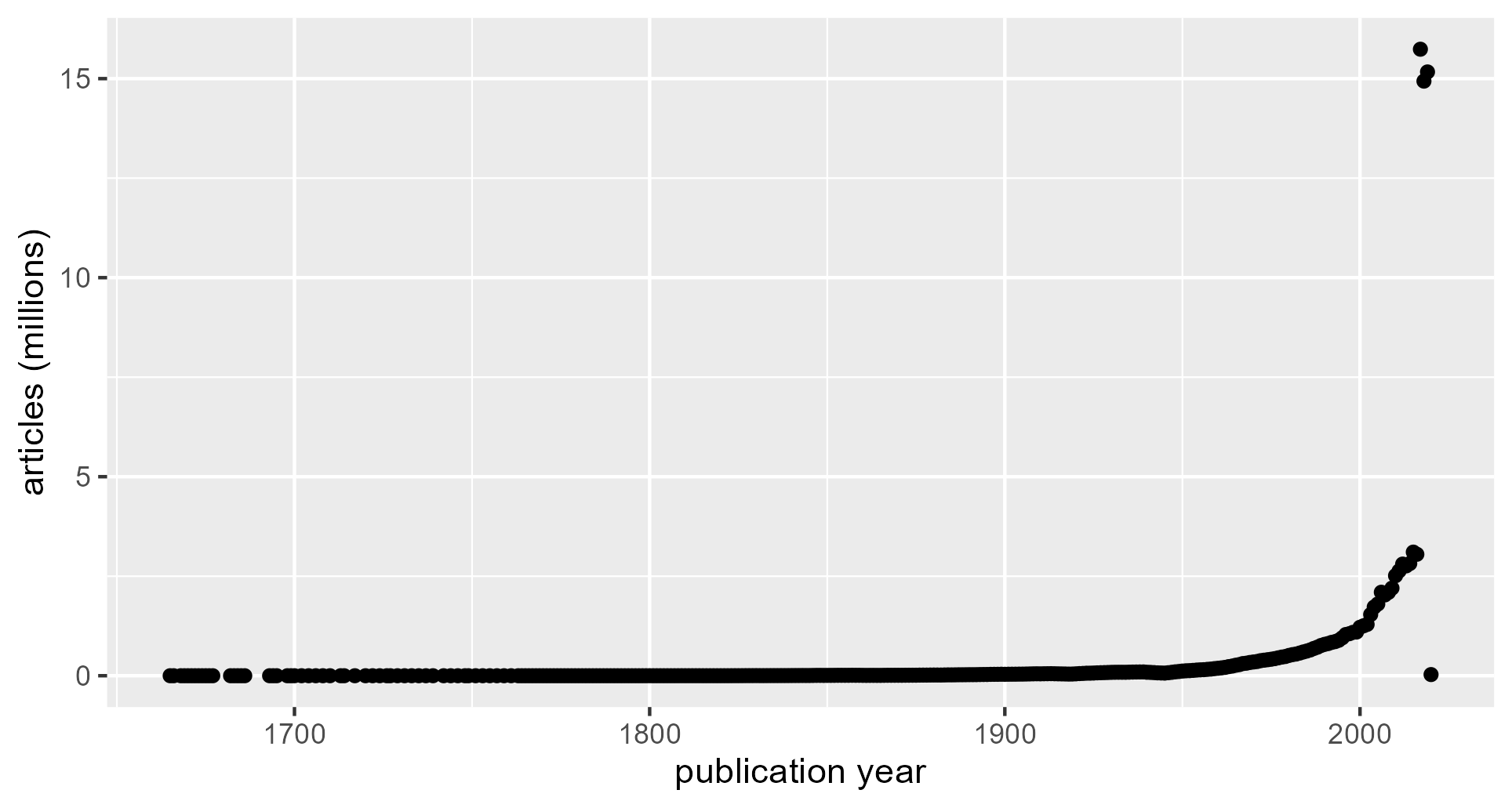
Figure 1. Number of articles per year.
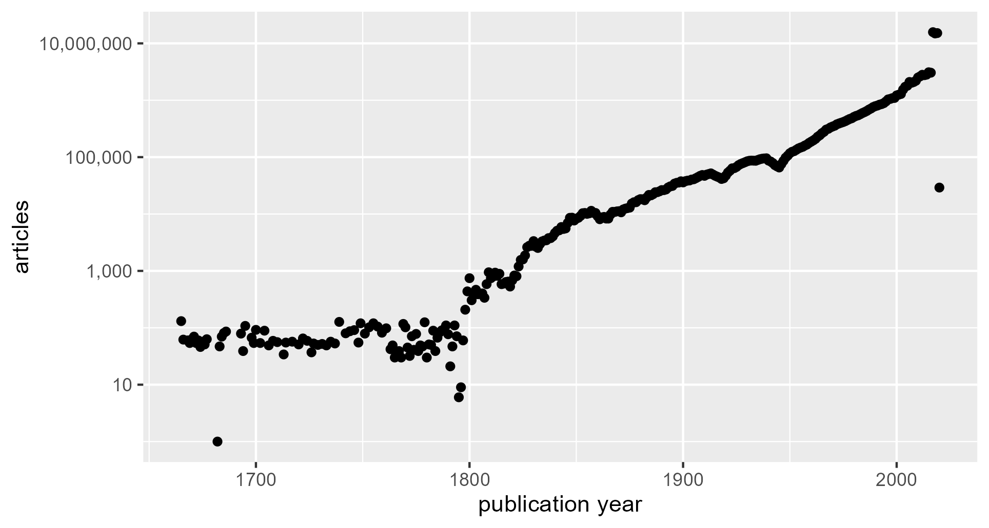
Figure 2. Number of articles per year, logarithmic scale.
The log scale makes several features of the data visually apparent: the absolute numbers during lower-volume publication years, the onset and duration of an exponential growth phase, and the publication burst in the most recent few years. The earliest publications in the GI (with realistic publication years) were produced in the 1660s. Thence forward, the GI contains on the order of 100 articles per year until 1880, when the article volume shows steady exponential growth through 2016. Article volume jumps by orders of magnitude in 2017. Low article volume in 2020 suggests that article accumulation ended in this year.
Local Workflow: literature indexing
The following diagram demonstrates the steps for compiling bibliographic information and determining yearly prevalence of a term in the GI.

Figure 3. GI workflow diagram. Functions and packages are shown in italics.
I performed these steps on a HP computer running Windows 10 with a 3.4 GHz Intel i3 CPU, 8 Gb RAM, 256 Gb internal hard drive, and an external 1 Tb hard drive. Scripts were written in R and run in RStudio.
Part I: file preparation
Download & Unzip
General Index files are available for download at https://archive.org/details/GeneralIndex. Downloading each keyword file and the single enhanced metadata file took roughly 6 hours apiece at a download speed of approximately 1 Mb/sec.
The zipped GI files require decompression before manipulation. To unzip the combined metadata file, I used the free utility 7-Zip (available at https://www.7-zip.org) twice: once to unpack the file from .gz to .tar, and again to yield a set of 16 .sql files.
To prepare the keyword files, I created an RStudio script that would individually decompress each file, search for terms of interest, retain the matches, and remove the expanded file before decompressing the next. This limited the amount of disk space needed to store keyword files to 457 Gb at any given time (355 Gb for all zipped slices + 102 Gb for the largest uncompressed file). If disk space is truly at a premium, it would be possible to download a single keyword file at a time, unzip it, extract records of interest, and delete the file before moving on to the next.
Part II: compiling a bibliography
Term search
Drosera is a genus of carnivorous plants (commonly known as Sundews) found on six continents [7]. To demonstrate literature indexing, I chose to search the GI keyword files for mentions of Sundew or Drosera.
The smallest decompressed keyword file was about 95 Gb, which was too large to read into Rstudio. However, the R function fread() (part of the data.table package) can pre- search a structured file and read in only the lines that match a particular pattern. This is done using the element “cmd” to execute an operating system command on the file before importing it into the RStudio environment. In this case, I used the pattern-searching command grep [8] to select lines that contained either ‘drosera’ or ‘sundew’. R could readily handle this data subset. To reduce exclusion of valid hits, I used a case-insensitive search and placed no restrictions on characters before or after each search string.
# -------- Creating a bibliography for search terms------------ #

## ---------- Unzip each file and read in keyword hits -------- ##

keyword_path = "D:/GI_files/keywords"
keyword_files = dir(keyword_path, pattern="*.sql.zip", full.names = TRUE)
keyword_headers = c("dkey", "keywords", "keywords_lc", "keyword_tokens",
                    "keyword_score", "doc_count", "insert_date")
keyword_tbl <- data.frame()


# -i makes the grep query case-insensitive
# -e makes the grep query an inclusive OR
query = str_c("-i -e 'drosera' -e 'sundew'")

for (i in keyword_files)
{
  expanded_file <- unzip(i, exdir="D:/GI_files")

  command = str_c("grep ", query, " ", expanded_file)
  current_tbl <- fread(cmd = command,
                       encoding="UTF-8",
                       quote="",
                       header=FALSE,
                       col.names = keyword_headers,
                       fill=TRUE,
                       keepLeadingZeros=TRUE)
  keyword_tbl <- rbind(keyword_tbl, current_tbl)

  file.remove(expanded_file)

  progress <- str_c("file ", i, " finished: ", Sys.time())
  print(progress)
}

write_tsv(keyword_tbl, "sundewkeywords.tsv")


## ------- Remove spurious hits, remove repeat articles ----- ##

dkey_list <- keyword_tbl %>%
    filter(!keywords %in% "Sundewall") %>%
    distinct(dkey)
The algorithm took roughly 50 minutes to process each slice (30 for unzipping and 20 for term matching), less than 14 hours total. It retrieved 9675 matching keyword records across the slices, which required less than 1 Mb of disk storage to save as a .tsv file.
At this stage it is prudent to manually inspect a sample of records to ensure the query behaves as intended. After looking at the results in OpenRefine [9], I added lines of code to filter the surname “Sundewall”, a spurious hit caught by my original query. I also included a line to remove duplicate instances in the dkey field. Duplicate article matches can occur even when searching for a single word, as GI keyword records may include the same term on its own and as part of one or more phrases. After these filtering steps, 4,565 unique articles remained.
Match Metadata
The next steps to turn this occurrence list into a useful index are to load in the GI metadata corresponding to the identified articles, using the common “dkey” field. I was unable to load the >4Gb metadata slice files into RStudio due to memory limitations. Instead, I made similar use of fread() and grep as with the keyword files, here reading in only the metadata records with dkey identifiers that matched the keyword hits. Since the search for each individual dkey occurred serially, this took considerable time – about 36 hours for the 4,565 unique Sundew dkeys. Metadata were found for 4336 (95.0%) of them.
## ------- Read in matching article metadata ---------------- ##

metadata_path = "D:/GI_files/metadata/doc_info.2022.12.update/doc_meta/doc_meta/"
meta_headers = c("dkey", "raw_id", "meta_key", "doc_doi", "meta_doi", "doi",
                 "doi_flag", "doi_status_detail", "doi_status", "isbn",
                 "journal", "doc_title", "meta_title", "title",
                 "doc_pub_date", "meta_pub_date", "pub_date",
                 "doc_author", "meta_author", "author",
                 "doc_size", "insert_date", "multirow_flag")
term_metadata <- data.frame()

dkeys_by_digit <- split(dkey_list, f=substr(dkey_list$dkey,1,1))
slice_list <- c(0:15)

for (slice in slice_list)
{
  file_path = str_c(metadata_path, "doc_meta_alt_", as.hexmode(slice), ".sql")
  dkey_vec <- as.data.frame(dkeys_by_digit[[slice+1]], col.names="dkey")

  for (i in dkey_vec$dkey)

  {
    query = str_c("-m 1 '^", i, "'")
    command = str_c("grep ", query, " ", file_path)
    current_tbl <- fread(cmd = command,
                         encoding="UTF-8",
                         quote="",
                         header=FALSE,
                         col.names = meta_headers,
                         sep="\t",
                         colClasses="character",
                         fill=TRUE,
                         keepLeadingZeros=TRUE)
    term_metadata <- rbind(term_metadata, current_tbl)

  }

    ## Optional - show progress bar for each slice
  progress <- str_c("Slice ", as.hexmode(slice), " finished: ", Sys.time())
  print(progress)
}
Table 3. First ten records of GI papers containing the terms “drosera” or “sundew”, reproduced as-is. Some metadata elements are hidden to improve readability. The full set is available at https://osf.io/s39n7/.
| title | author | pub_date | journal | isbn | doi |
|---|---|---|---|---|---|
| EDIT PAGE 20 | N/A | 8/7/2015 | \N | \N | N/A |
| Mycorrhizal Status of Knieskern’s Beaked Sedge (Rhynchospora knieskernii) in the New Jersey Pine Barrens | John Dighton, Ted Gordon, Rosa Mejia and Marilyn Sobel | 2013 | Bartonia | 10.2307/41955392 | |
| REVIEWS OF BRITISH AND FOREIGN LITERATURE. The Natural History of Digestion | A Lockhart Gillespie; London; Walter Scott | 2/16/2019 | \N | \N | N/A |
| Notes on the Flora of Block Island | W. W. Bailey | 1893-06-17 | Bulletin of the Torrey Botanical Club | 10.2307/2475918 | |
| Cytological analysis of ginseng carpel development | Silva, Jeniffer; Kim, Yu-Jin; Xiao, Dexin; Sukweenadhi, Johan; Hu, Tingting; Kwon, Woo-Saeng; Hu, Jianping; Yang, Deok-Chun; Zhang, Dabing | 2/2/2017 | Protoplasma | 10.1007/s00709-017-1081-4 | |
| Caryophyllales: a key group for understanding wood anatomy character states and their evolutionb oj_1095 342..393 | Sherwin Carlquist Fls | 8/11/2017 | \N | \N | N/A |
| Frederick Burkhardt; James Secord;\\r <i>et al.</i>\\r (Editors).\\r <i>The Correspondence of Charles Darwin</i>\\r . Volume 20. xxxix + 862 pp., illus., bibl., index. Cambridge: Cambridge University Press, 2013. £90 (cloth).Frederick Burkhardt; James Secord;\\r <i>et al.</i>\\r (Editors).\\r <i>The Correspondence of Charles Darwin</i>\\r . Volume 21. xxxvii + 784 pp., illus., bibl., index. Cambridge: Cambridge University Press, 2014. £90 (cloth). | Ghiselin, Michael | 12/2/2015 | Isis | 10.1086/684657 | |
| Structure Elucidation of Plumbagin Analogues from\\r <i>Dionea muscipula</i>\\r and their\\r <i>in vitro</i>\\r Immunological Activity on Human Granulocytes and Lymphocytes | Kreher, B.; Neszmelyi, A.; Polos, K.; Wagner, H. | 1989-2 | Planta Medica | 10.1055/s-2006-961890 | |
| Trading in Genes. Development Perspectives on Biotechnology, Trade and Sustainability | Van Damme, Patrick | 2006-12 | Economic Botany | 10.1663/0013-0001(2006)60[394b:tigdpo]2.0.co;2 | |
| Flowers of July and August | Edward H. Day | 1879-08 | The Art Amateur | 10.2307/25626849 |
The article metadata show inconsistent formatting, sporadic inclusion of markup, and missing information. Nonetheless, in most cases there is sufficient information to identify each article.
One could ask what advantages this method has over searching for papers in Google Scholar. The analogous query (drosera* or Sundew*) yielded 6,140 results (search performed on Jun 2, 2023) – admittedly a larger number than found in the General Index. However, Google Scholar records cannot be exported in bulk. Also, not all articles and citations in Google Scholar have searchable full text [10]. Since neither database fully encompasses the scholarly literature, searching the General Index could complement searches in Google Scholar.
Part III: yearly term prevalence
Select publication dates
Reporting the number of articles per year containing a given term is not useful for determining the term’s prevalence over time, as it does not account for the total number of articles in the general index for that year. Finding the total is challenging in a limited computing setting, because each single metadata slice is too large to read fully into R.
I overcame this limitation with another application of fread(). I used a command to accomplish two tasks on each line of the file before reading in the data: select lines that contain metadata records (to avoid reading in SQL header information) and read in only the columns needed for the current task.
To accomplish this, I settled on a statement in the awk [11] programming language [12]. The statement selects lines that begin with a 40-character hexadecimal number (corresponding to a valid dkey), then returns the fields corresponding to the dkey and publication date [13]. This allowed reading in dkey/publication date pairs at a rate of 2-3 minutes per slice, or about 40 minutes total.
# ------ Calculate Yearly Term Prevalence --------------- #

## ------- Get years for all metadata ------------------ ##

date_headers = c("dkey", "pub_date")
slice_list <- c(0:15)
count_tbl <- list()

for (slice in slice_list)
{
  file_path = str_c(metadata_path, "doc_meta_alt_", as.hexmode(slice), ".sql")

  expression = str_c("/^[0-9a-f]{40,}/") # find lines starting with 40 hex characters
  command = str_c("awk ' BEGIN {FS=OFS=\"\t\"} $1 ~ ",
                  expression, " {print $1, $17} ' ", file_path)

  current_tbl <- fread(cmd = command,
                      encoding="UTF-8",
                      quote="",
                      header=FALSE,
                      col.names = date_headers,
                      sep="\t",
                      fill=TRUE,
                      keepLeadingZeros=TRUE)

  # Detect four consecutive integers in the publication date field to determine year
  current_tbl <- current_tbl %>%
    mutate(pub_year = str_extract(pub_date, '[0-9]{4,}'))


  count_tbl[[slice+1]] <- count(current_tbl, pub_year)

  ## Optional - show progress bar for each slice
  progress <- str_c("Slice ", as.hexmode(slice), " finished: ", Sys.time())
  print(progress)
}

meta_dates <- do.call("rbind", count_tbl) %>%
 count(pub_year, wt=n)
I encountered memory constraints when trying to combine the dkey/publication date information across all slices. Instead, I had the script count the number of GI articles for each year for each slice individually without retaining the raw dkey/publication date information, and later totaled the year counts across slices.
Spurious hits are unlikely at this stage. The dkey identifier is assigned to articles by applying a hash algorithm to yield a 40-digit hexadecimal number. Thus, there are 1640 (1.5 * 1048) possible unique results of this hash. The probability that the set of 1.1*108 articles contains at least one pair of different articles with the same hash is roughly 3 * 10-23 [14].
Determine Year
The GI metadata table contains three fields with information about publication year: doc_pub_date (publication date extracted from the document text), meta_pub_date (publication date given in document metadata), and pub_date (date from metadata if available, text if not). I chose to determine dates from the pub_date field to give the greatest likelihood of successful extraction.
Date formats are not standardized in the GI – months and days are not always given, and the order and separating characters may vary. I focused on the four-digit year to avoid confusion among ways to format dates and provide a convenient unit for diachronic analysis. For both the metadata and keyword bibliographic data, I used the R stringr function str_extract() to detect when four consecutive digits were present in the pub_date field and add them to a new field, pub_year.
Count & Normalize
The Rstudio package dplyr contains convenient functions to count() occurrences in data columns and mutate() columns to perform arithmetic operations. I used count() on the pub_year field to determine the total number of articles per year in the GI, and number of articles per year in the keyword hit subset. I joined these results into a new table by the common field of publication year, then calculated a new field called “prevalence” by dividing the count of articles containing the term by the count of articles in the GI for that year.
## ------- Determine term publication years,

## ------ Count and normalize -------------------------- ##

term_pub_year <- arranged_results %>%
  mutate(pub_year = str_extract(pub_date, '[0-9]{4,}')) %>%
  count(pub_year) %>%
  left_join(meta_dates, join_by(pub_year), suffix=c(".t", ".m")) %>%
  mutate(prevalence = n.t/n.m) %>%
  arrange(pub_year)
Visualize
## ------- Plot prevalence by year --------------------- ##

prevalence_plot <- ggplot(data=term_pub_year,
                          aes(x=as.integer(pub_year), y=prevalence)) +
                          scale_y_break(c(0.0015, 0.013), space = 0.8) +
                          labs(x="publication year", y="prevalence (percentage)") +
                   geom_point()

prevalence_plot
Plotting the prevalence term over time is a proxy for interest in the term over time. The plot of Sundews shows the species has not had a resurgence of interest since a series of upticks in the 1870s and the early 1900s.
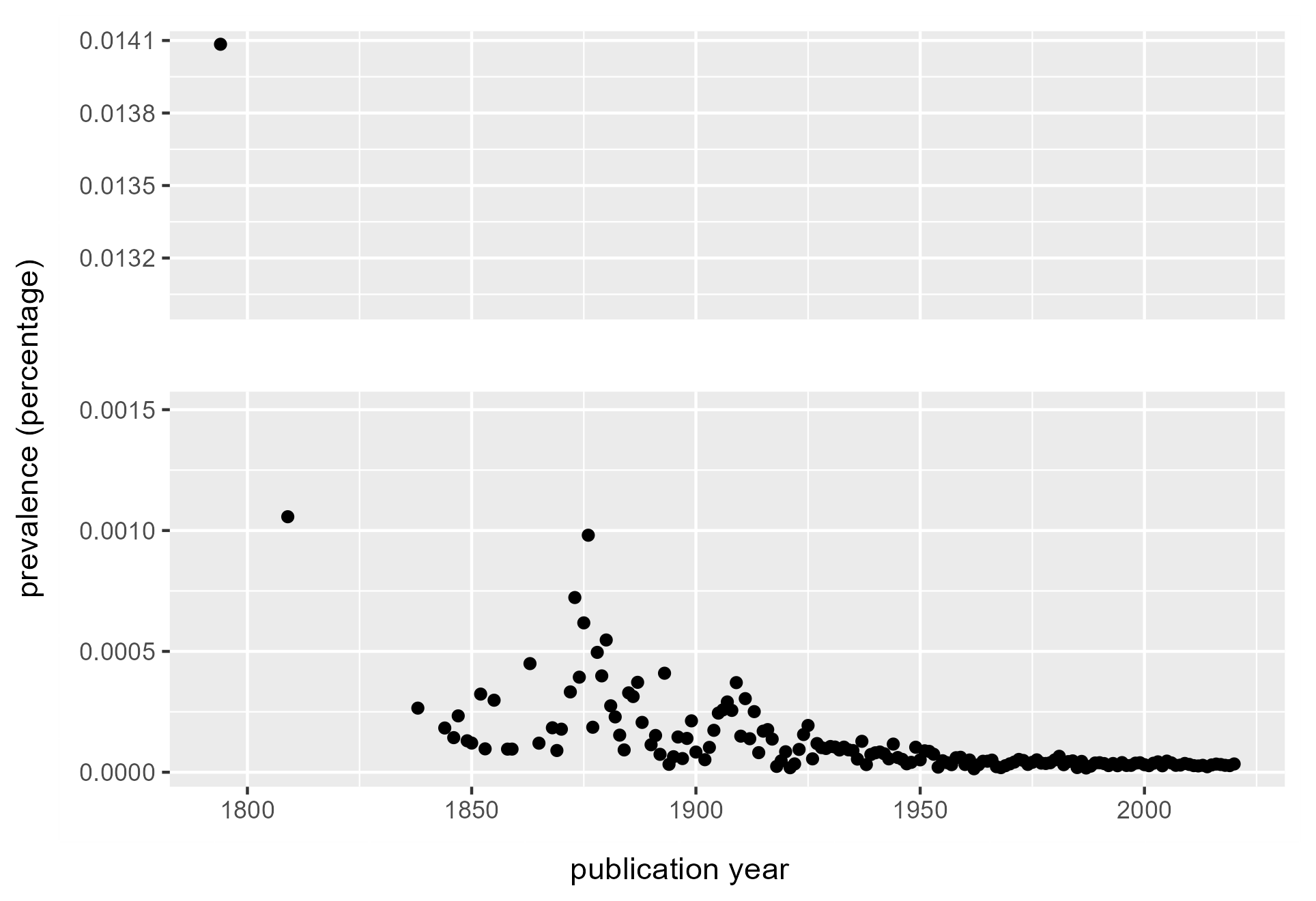
Figure 4. Prevalence of the terms “sundew” or “drosera” in the General index. Starting from 1850 onward, sundews see the greatest representation around 1875, with spikes of interest around 1910 and 1925. From then their prevalence stays relatively consistent, suggesting little special attention paid beyond a baseline interest. Earlier data are more noisy, and sparse hits before 1825 suggest too little data to interpret.
These results may appear similar to a Google Ngram viewer plot, but they measure publication volume in different ways, making direct comparison inappropriate. In the above, prevalence shows the proportion of articles in the GI containing at least one mention of the desired term. Google Ngram Viewer plots frequency, the proportion of occurrences of a word/term normalized by total number of words in the corpus per year. A more comparable method is to download raw data from the Google Ngram corpus, which allows a similar calculation of yearly prevalence – as the proportion of volumes in Google Books containing a term, compared to the total volumes in the Google Books corpus. However, this is only possible if looking for a single term of interest; in the example above, volumes containing both “sundew” and “drosera” would be double-counted.
HPC adaptations
I performed my first explorations of the General Index on Kamiak, the Washington State University high performance computing cluster. Only after becoming familiar with the data set and potential workflows was I able to devise the local approach described above, which I hope will be accessible to more researchers. Working in a high-performance computing environment confers multiple advantages that boil down to: doing more things, faster. An HPC can manipulate the ngram files, run multiple queries in parallel, and accomplish individual tasks faster than less powerful computers. Scripts used to process and analyze the data can be more straightforward, as they do not require memory restriction workarounds.
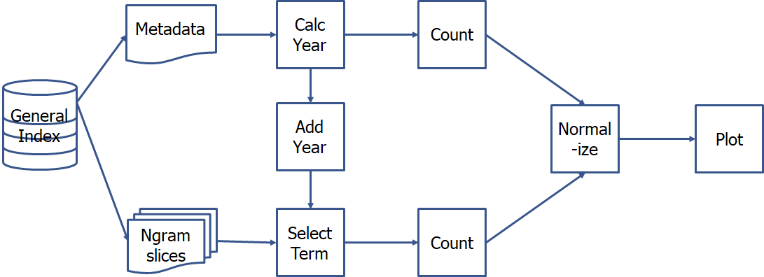
Figure 5. HPC workflow for creating a yearly ngram prevalence plot
Kamiak includes 500 Gb of storage space per lab with a free-tier account and temporary (up to two weeks) scratch storage of 10 Tb. Access to this scratch storage let me serially download, unzip, and query ngram slices, then save the results to permanent storage.
Kamiak runs a Linux operating system that I accessed using the Windows Subsystem for Linux Ubuntu application. In this environment one can use scripts to perform simple file and table manipulations, perform multiple tasks in sequence, and run tasks in parallel using job arrays. This makes it easy to search for multiple keywords or ngrams at the same time and later combine and compare the results.
I downloaded files directly from the GI using the Linux command wget and extracted them with the commands unzip (for .zip files) and tar (for .tar.gz metadata files). In a series of bash scripts, I appended metadata years to all the metadata records, used grep and regular expressions to select ngram records that contained my search terms of interest. I used R scripts similar to those described in the desktop sections to count occurrences of publication years, normalize by article years across the corpus, and plot the results. I ran the R scripts on Kamiak when the search result files were too large to read into Rstudio locally. I intend to present more details on these processes in a future publication.
Discussion
This paper shows that working with the General Index is feasible in a desktop computing environment, so long as we:
- Limit the analysis to the keyword and metadata files
- Retrieve a sufficiently small number of keyword hits
- Employ R packages that can selectively read subsets of file data into memory.
Applied to the GI, these methods can create bibliographies and diachronic analyses of keywords used throughout the history of academic publishing. Though beyond the scope of this work, one could imagine performing a more nuanced analysis by incorporating the YAKE (“meaningfulness”) score to include a dimension of relative importance of the keyword in each article.
If working in an HPC environment, analyzing ngrams would allow querying longer phrases and greatly increase the number of results retrieved – hits would not be limited by their importance in the document. Using these longer phrases would also facilitate the use of additional text and data mining analytic methods, such as colocation and topic modeling.
This paper presents one method for searching the General Index, but it is by no means the only way. All the tasks I have described are straightforward [15] file and text manipulations confounded by the size of the data set. Any software or method that can perform similar manipulations is fine for the purpose. I hope this paper will inspire others to explore and experiment with this resource. For those that do, here are a few considerations:
- When possible, subdivide large data sets and work on smaller chunks. Test code on very small data subsets to avoid long wait times to verify the desired effect.
- Strive for consistency in file formats and encoding. Choose conventions for importing and exporting files (e.g., UTF-8 encoding, tab-separated file format), and use them throughout the workflow.
- General Index files can also be downloaded via torrent, which could be faster and more resilient to interruption. Local campus policy prohibited me from testing this.
- The R package SQLite may offer other methods and shortcuts for querying large files in R. I did not test this approach due to unfamiliarity.
Admittedly, the limitations of the General Index go beyond its lack of interface. Even my sample metadata records show a substantial lack of data cleaning, missing fields, and inconsistent formats and standards. Five percent of article identifiers in the sundew sample lacked corresponding metadata altogether. One should take this uncertainty into account when choosing analyses to conduct and interpreting results.
There is also little transparency in how well the articles in the GI constitute a representative sample of the entire universe of published articles. It is possible to determine the distribution of publication dates, but it is much harder to characterize the articles in other ways. Articles in languages other than English are present but sparse. The methods used to collect the articles could over- or underrepresent different article types, disciplines, or knowledge domains. It is difficult to infer the direction and possible extent of bias without more information about the origins of the articles within the GI, and this limits the extent we can responsibly interpret and draw conclusions from the data.
The stability of the resource is also unclear, as the database’s legality has not yet been tested. Malamud maintains that the GI does not infringe copyright despite containing information derived from paywalled papers, because the text is only retrievable in short fragments [16]. However, the legality of amassing the articles in the first place is unclear [17].
Currency is also a factor in the GI’s utility. According to Carl Malamud, the database is planned to be updated yearly at most [18].
These caveats are substantial, but I still consider the GI highly valuable because it opens up the scholarly record to an extent of inquiry that was previously impossible, and does so freely to the public. It can aid in comprehensive literature searching, following concepts over time, and text mining. By focusing on local computing workflows, I hope this paper can reach a broad and diverse audience of researchers, who will in turn ask a broad variety of questions of the scholarly record. I am eager to collaborate with others interested in working with this database and happy to offer advice for using it.
Acknowledgements
This paper would not be possible without the hard work of Carl Malamud and Public Resource to create the General Index in the first place, and making it available to the public. I offer many thanks to Elizabeth Blakesley and Jay Starratt for encouraging me to follow my research interests, wherever they may roam. Thanks also to Elizabeth Blakesley, Suzanne Fricke, Ann Dyer, Clara del Junco, and Xanda Schofield for helpful conversations on this work and resource, and all my WSU library colleagues for moral support. Many thanks to the Kamiak HPC/WSU Center for Institutional Research Computing (CIRC) https://hpc.wsu.edu for unhesitatingly providing access to the HPC cluster that enabled this work and for kind troubleshooting assistance. This work was not supported by grant funding.
About the Author
Emily Cukier (ORCID ID: 0000-0002-3972-5506) has been a Science Librarian at Washington State University since October 2021.
References and Notes
[1] In this context, “keywords” do not refer to key terms/phrases assigned by an author or editors to aid finding, but words or short phrases identified by an importance-scoring algorithm.
[2] The General Index. 2021. [accessed 2023 Jul 7]. http://archive.org/details/GeneralIndex.
[3][5][17] Pulla P. 2019. The plan to mine the world’s research papers. Nature. 571(7765):316–318. doi:10.1038/d41586-019-02142-1.
[4][16] Else H. 2021. Giant, free index to world’s research papers released online. Nature. doi:10.1038/d41586-021-02895-8. [accessed 2023 Apr 24]. https://www.nature.com/articles/d41586-021-02895-8.
[6] Campos R, Mangaravite V, Pasquali A, Jorge A, Nunes C, Jatowt A. 2020. YAKE! Keyword extraction from single documents using multiple local features. Inf Sci. 509:257–289. doi:10.1016/j.ins.2019.09.013.
[7] Barthlott W, Ashdown M. 2007. The curious world of carnivorous plants : a comprehensive guide to their biology and cultivation. English language ed. Portland, Or: Timber Press.
[8] The grep command is used with regular expressions and can perform far more sophisticated pattern-matching than is described here. One good tool for learning and experimenting with regular expressions is available at https://regexr.com.
[9] OpenRefine is a free data viewing and wrangling tool available at https://openrefine.org/.
[10] Lopez-Cozar ED, Orduna-Malea E, Martin-Martin A, Ayllon JM. 2018. Google Scholar: the “big data” bibliographic tool. doi:10.48550/arXiv.1806.06351. [accessed 2023 May 30]. http://arxiv.org/abs/1806.06351.
[11] AWK (named after creators Alfred Aho, Peter Weinberger, and Brian Kernighan), is a scripting language highly suited for pattern matching in structured data.
[12] Aho AV, Kernighan BW, Weinberger PJ. 1988. The AWK programming language. Reading, Mass: Addison-Wesley Pub. Co. (Addison-Wesley series in computer science).
[13] These fields correspond to the first and seventeenth columns in metadata file version 10.21. The field indexes may require updates if later metadata file versions change the order or number of columns.
[14] Calculation performed at https://www.bdayprob.com with D=1640 (entered as 2128) and N=1.1*108 (approximated and entered as 227)
[15] I admit that straightforwardness is in the eye of the beholder.
[18] Carl Malamud, personal communication

Subscribe to comments: For this article | For all articles
Leave a Reply